iDEP is a tool for interactive analysis of RNA-Seq data. After analyzing their data, users have the option to download a R Markdown file, toegether with other data files, to reproduce the entire workflow. This blog is both the easiest and the hardest of all. It is easy because everything below was automatically generated by iDEP; it is hard as I have to write code to write code when developing iDEP.
1. Read data
R packages and iDEP core Functions. Users can also download the iDEP_core_functions.R file. Many R packages needs to be installed first. This may take hours. Each of these packages took years to develop.So be a patient thief. Sometimes dependencies needs to be installed manually. If you are using an older version of R, and having trouble with package installation, try un-install the current version of R, delete all folders and files, and reinstall from scratch.
 if(file.exists('iDEP_core_functions.R'))
	source('iDEP_core_functions.R') else
    source('https://raw.githubusercontent.com/iDEP-SDSU/idep/master/shinyapps/idep/iDEP_core_functions.R')
We are using the downloaded gene expression file where gene IDs has been converted to Ensembl gene IDs. This is because the ID conversion database is too large to download. You can use your original file if your file uses Ensembl ID, or you do not want to use the pathway files available in iDEP (or it is not available).
 inputFile <- 'C:/Users/Xijin.Ge/Downloads/Downloaded_Converted_Data.csv'  # Expression matrix
 sampleInfoFile <- 'C:/Users/Xijin.Ge/Downloads/Downloaded_sampleInfoFile.csv' # Experiment design file
 geneInfoFile <- 'C:/Users/Xijin.Ge/Downloads/Mouse__mmusculus_gene_ensembl_GeneInfo.csv' #Gene symbols, location etc.
 geneSetFile <- 'C:/Users/Xijin.Ge/Downloads/Mouse__mmusculus_gene_ensembl.db'  # pathway database in SQL; can be GMT format
 STRING10_speciesFile <- 'https://raw.githubusercontent.com/iDEP-SDSU/idep/master/shinyapps/idep/STRING10_species.csv'
Parameters for reading data
 input_missingValue <- 'geneMedian'	#Missing values imputation method
 input_dataFileFormat <- 1	#1- read counts, 2 FKPM/RPKM or DNA microarray
 input_minCounts <- 0.5	#Min counts
 input_NminSamples <- 1	#Minimum number of samples
 input_countsLogStart <- 4	#Pseudo count for log CPM
 input_CountsTransform <- 1	#Methods for data transformation of counts. 1-EdgeR's logCPM 2-VST, 3-rlog
 readData.out <- readData(inputFile)
 library(knitr)   #  install if needed. for showing tables with kable
 kable( head(readData.out$data) )    # show the first few rows of data
| p53_mock_1 | p53_mock_2 | p53_mock_3 | p53_mock_4 | p53_IR_1 | p53_IR_2 | p53_IR_3 | p53_IR_4 | null_mock_1 | null_mock_2 | null_IR_1 | null_IR_2 | |
|---|---|---|---|---|---|---|---|---|---|---|---|---|
| ENSMUSG00000075014 | 5.986190 | 10.245204 | 11.622005 | 12.445437 | 19.58986 | 21.07925 | 8.279954 | 17.40506 | 13.23741 | 12.91427 | 6.949322 | 14.57512 |
| ENSMUSG00000076617 | 18.174331 | 18.020764 | 17.901045 | 16.892389 | 18.06544 | 18.52019 | 16.933927 | 17.68636 | 17.18909 | 17.39665 | 17.663020 | 17.21374 |
| ENSMUSG00000015656 | 15.349228 | 15.086274 | 15.392536 | 14.817324 | 15.95674 | 15.75896 | 16.233039 | 16.04712 | 15.03582 | 14.98886 | 18.603855 | 17.00075 |
| ENSMUSG00000052305 | 13.766147 | 11.436670 | 10.523028 | 15.927563 | 10.57175 | 11.22625 | 10.125088 | 10.20851 | 11.81668 | 17.59129 | 10.311098 | 15.82093 |
| ENSMUSG00000069917 | 13.511114 | 11.202619 | 10.240337 | 15.915347 | 10.33765 | 11.20676 | 10.280270 | 10.32910 | 11.51218 | 17.41403 | 10.236792 | 15.73450 |
| ENSMUSG00000075015 | 4.023733 | 7.791965 | 9.161421 | 9.809036 | 16.98655 | 18.47457 | 5.767006 | 14.96939 | 10.59269 | 10.25800 | 4.742948 | 12.00540 |
 readSampleInfo.out <- readSampleInfo(sampleInfoFile)
 kable( readSampleInfo.out )
| p53 | Treatment | |
|---|---|---|
| p53_mock_1 | wt | mock |
| p53_mock_2 | wt | mock |
| p53_mock_3 | wt | mock |
| p53_mock_4 | wt | mock |
| p53_IR_1 | wt | IR |
| p53_IR_2 | wt | IR |
| p53_IR_3 | wt | IR |
| p53_IR_4 | wt | IR |
| null_mock_1 | null | mock |
| null_mock_2 | null | mock |
| null_IR_1 | null | IR |
| null_IR_2 | null | IR |
 input_selectOrg ="NEW"
 input_selectGO <- 'KEGG'	#Gene set category
 input_noIDConversion = TRUE
 allGeneInfo.out <- geneInfo(geneInfoFile)
 converted.out = NULL
 convertedData.out <- convertedData()
 nGenesFilter()
## [1] "6882 genes in 12 samples. 6882 genes passed filter.\n Original gene IDs used."
 convertedCounts.out <- convertedCounts()  # converted counts, just for compatibility
 readCountsBias()  # detecting bias in sequencing depth
## [1] "Warning! Sequencing depth bias detected. Total read counts are significantly different among sample groups (p= 1.04e-02 ) based on ANOVA."
2. Pre-process
# Read counts per library
 parDefault = par()
 par(mar=c(12,4,2,2))
 # barplot of total read counts
 x <- readData.out$rawCounts
 groups = as.factor( detectGroups(colnames(x ) ) )
 if(nlevels(groups)<=1 | nlevels(groups) >20 )
  col1 = 'green'  else
  col1 = rainbow(nlevels(groups))[ groups ]

 barplot( colSums(x)/1e6,
		col=col1,las=3, main="Total read counts (millions)")
 # Box plot
 x = readData.out$data
 boxplot(x, las = 2, col=col1,
    ylab='Transformed expression levels',
    main='Distribution of transformed data')
 #Density plot
 par(parDefault)
 densityPlot()
 # Scatter plot of the first two samples
 plot(x[,1:2],xlab=colnames(x)[1],ylab=colnames(x)[2],
    main='Scatter plot of first two samples')
####plot gene or gene family
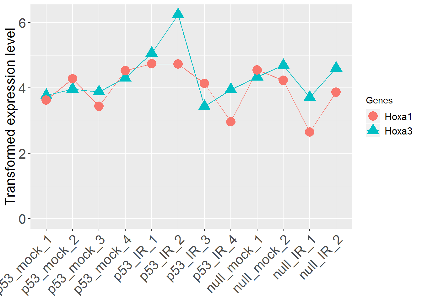
input_selectOrg ="BestMatch"
input_geneSearch <- 'HOXA' #Gene ID for searching
genePlot()
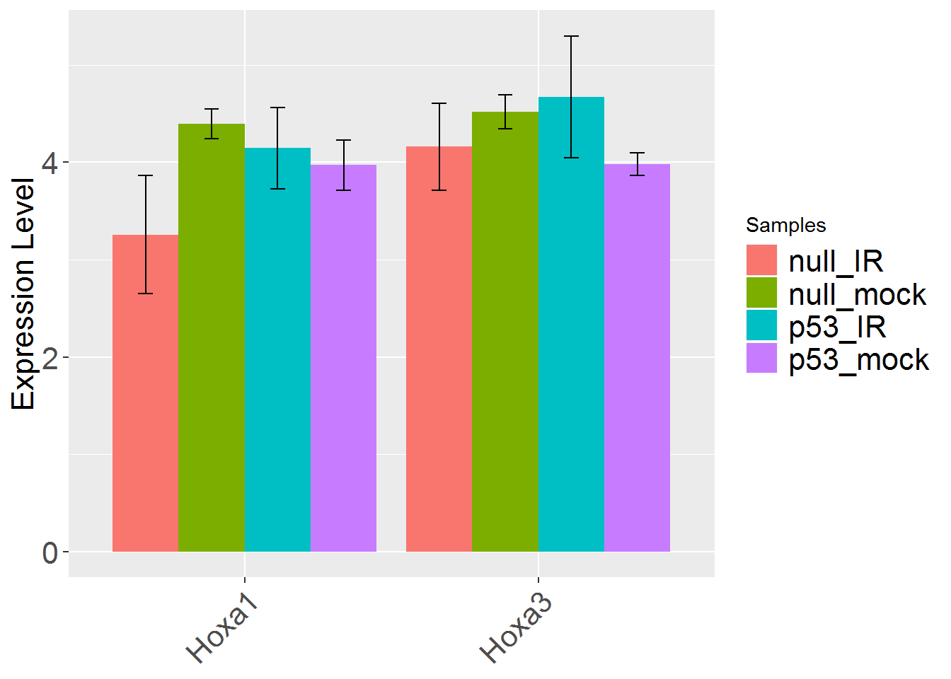
 input_useSD <- 'FALSE'	#Use standard deviation instead of standard error in error bar?
 geneBarPlotError()
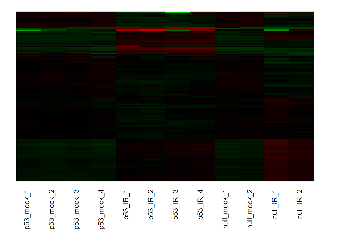
3. Heatmap
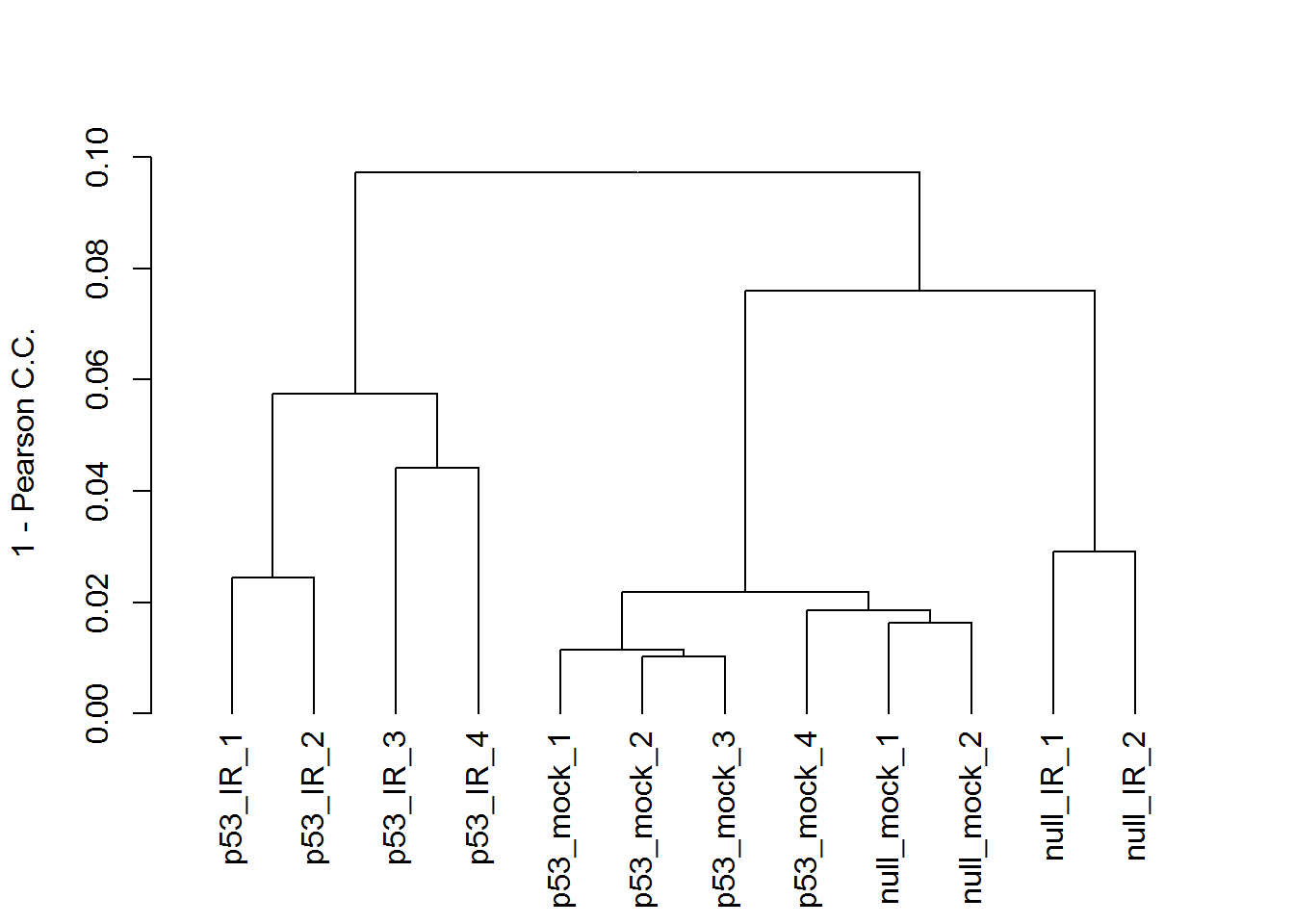
 # hierarchical clustering tree
 x <- readData.out$data
 maxGene <- apply(x,1,max)
 # remove bottom 25% lowly expressed genes, which inflate the PPC
 x <- x[which(maxGene > quantile(maxGene)[1] ) ,]
 plot(as.dendrogram(hclust2( dist2(t(x)))), ylab="1 - Pearson C.C.", type = "rectangle")
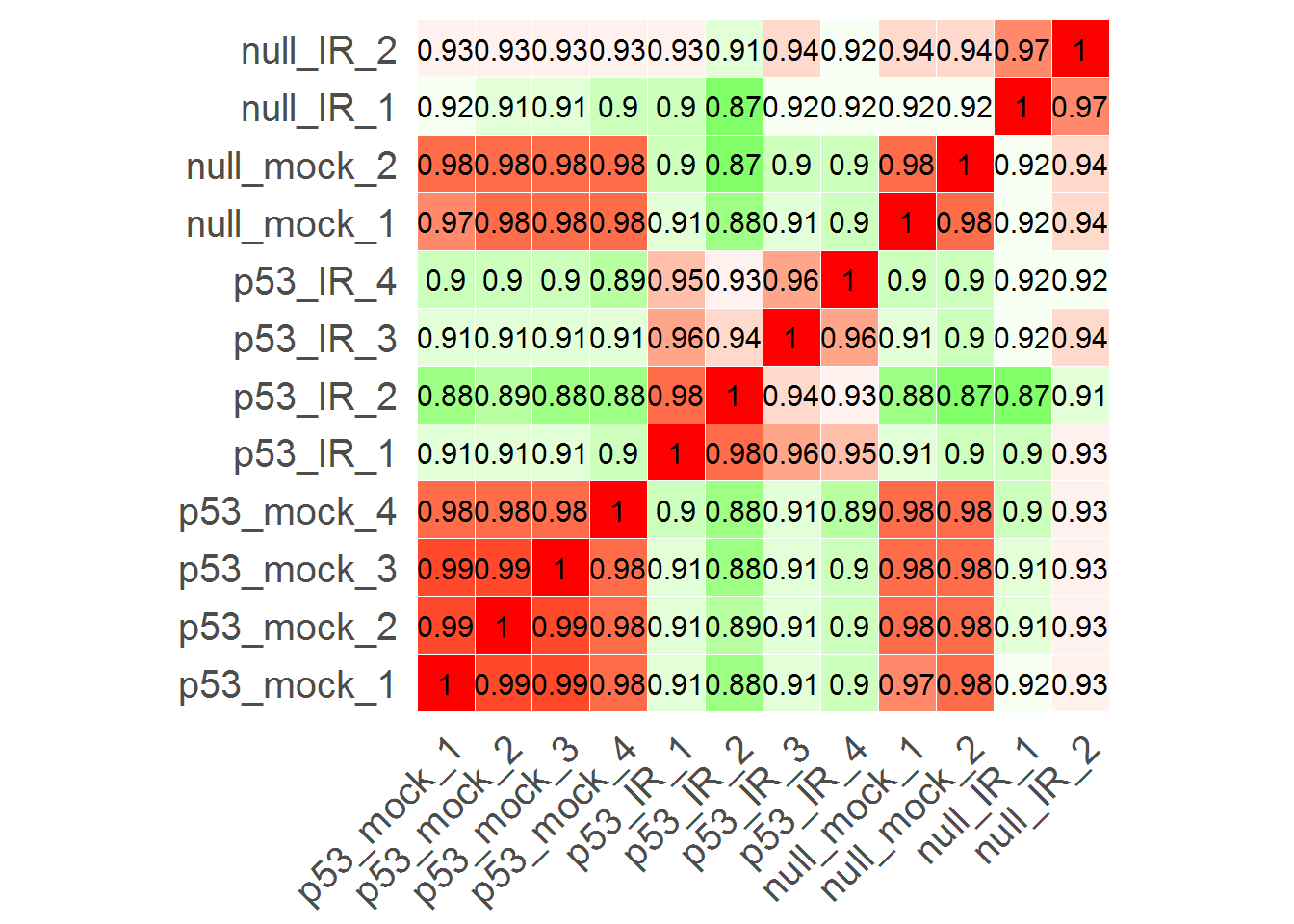
 #Correlation matrix
 input_labelPCC <- TRUE	#Show correlation coefficient?
 correlationMatrix()
 # Parameters for heatmap
 input_nGenes <- 1000	#Top genes for heatmap
 input_geneCentering <- TRUE	#centering genes ?
 input_sampleCentering <- FALSE	#Center by sample?
 input_geneNormalize <- FALSE	#Normalize by gene?
 input_sampleNormalize <- FALSE	#Normalize by sample?
 input_noSampleClustering <- FALSE	#Use original sample order
 input_heatmapCutoff <- 4	#Remove outliers beyond number of SDs
 input_distFunctions <- 1	#which distant funciton to use
 input_hclustFunctions <- 1	#Linkage type
 input_heatColors1 <- 1	#Colors
 input_selectFactorsHeatmap <- 'Sample_Name'	#Sample coloring factors
 #png('heatmap.png', width = 10, height = 15, units = 'in', res = 300)
 #staticHeatmap()
 #dev.off()
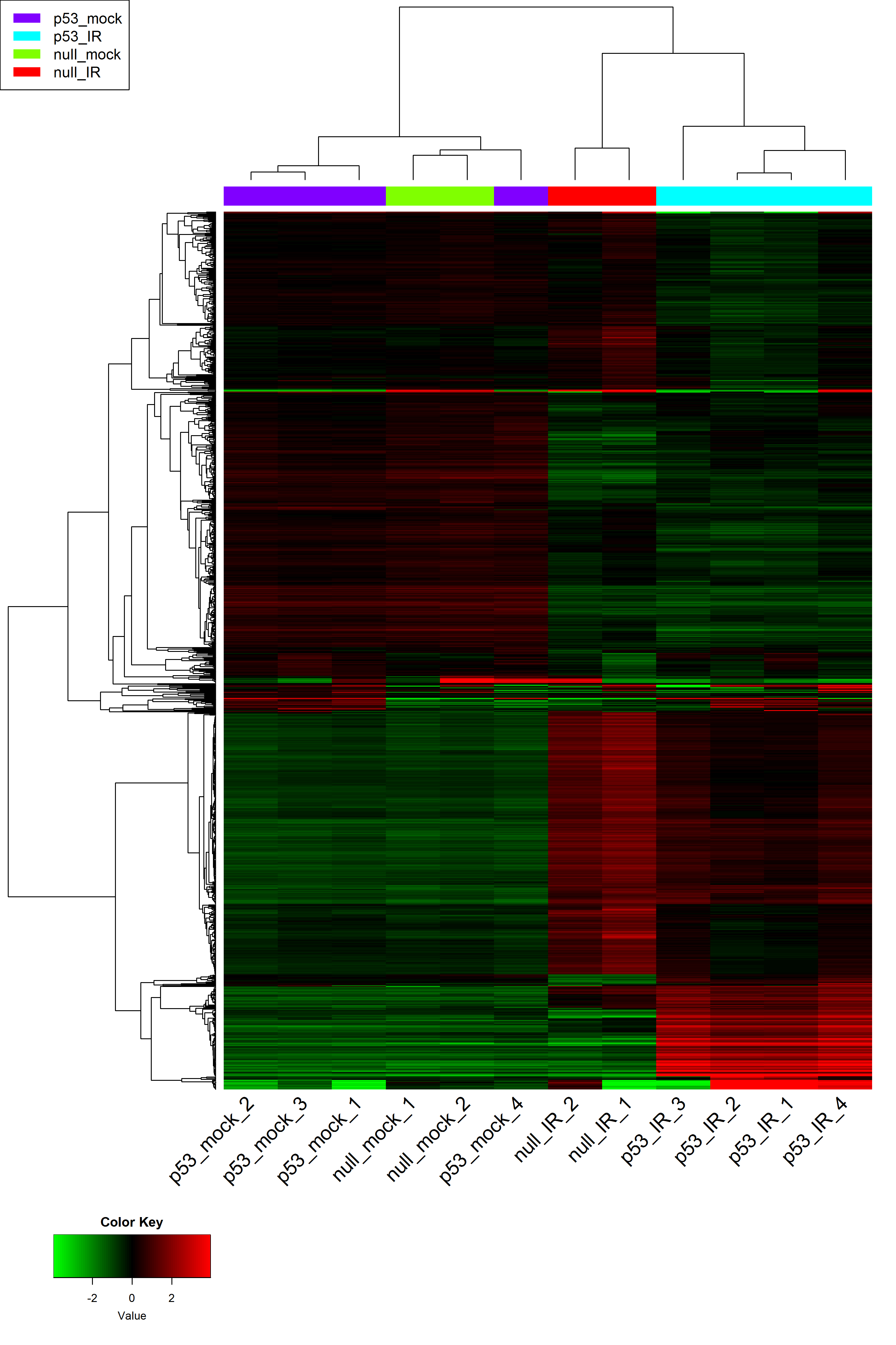
# heatmapPlotly() # interactive heatmap using Plotly
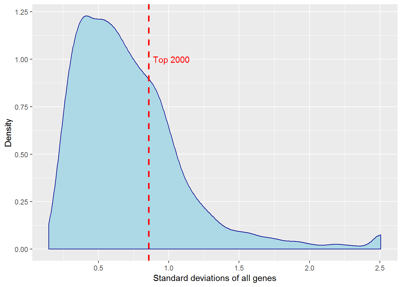
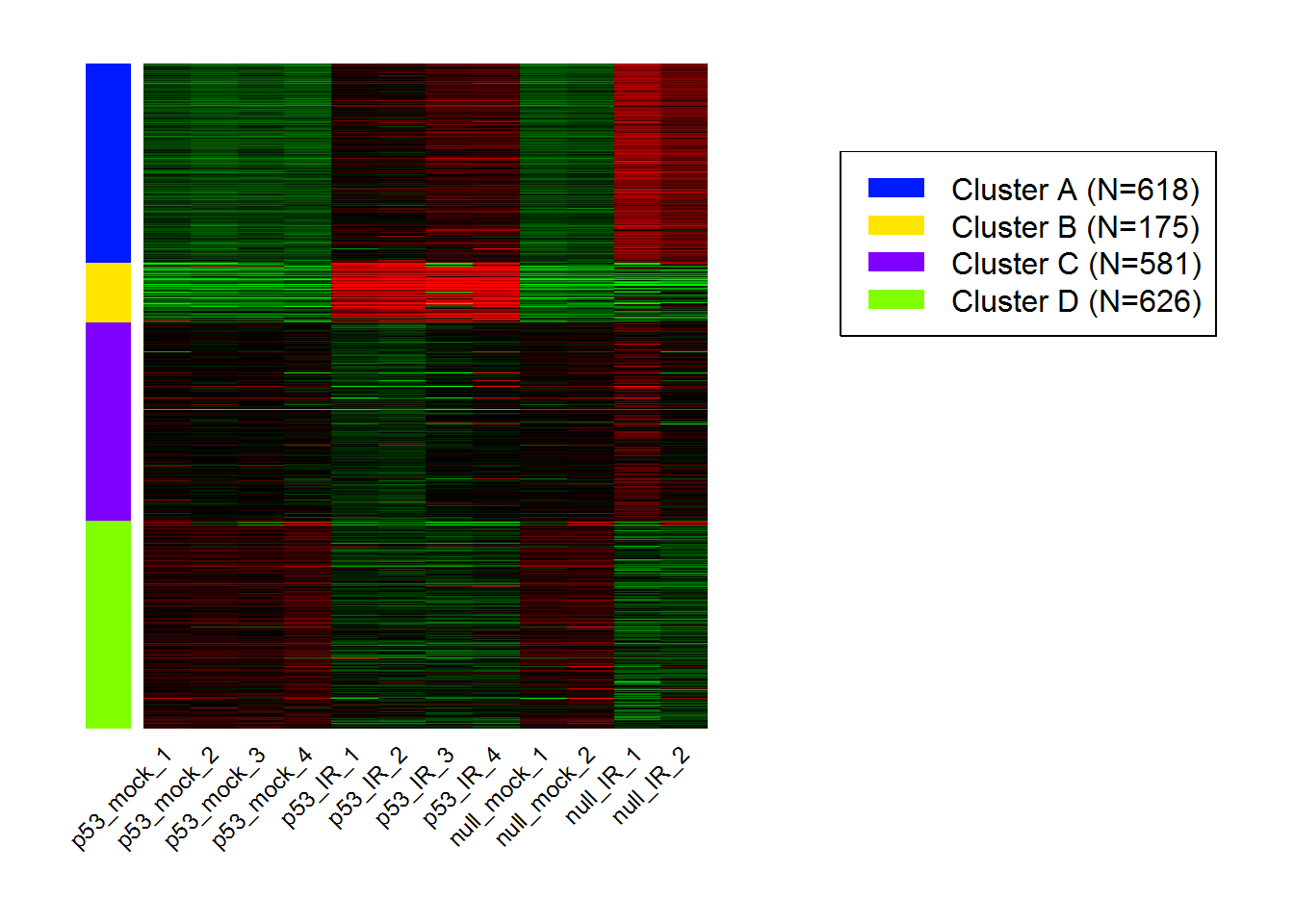
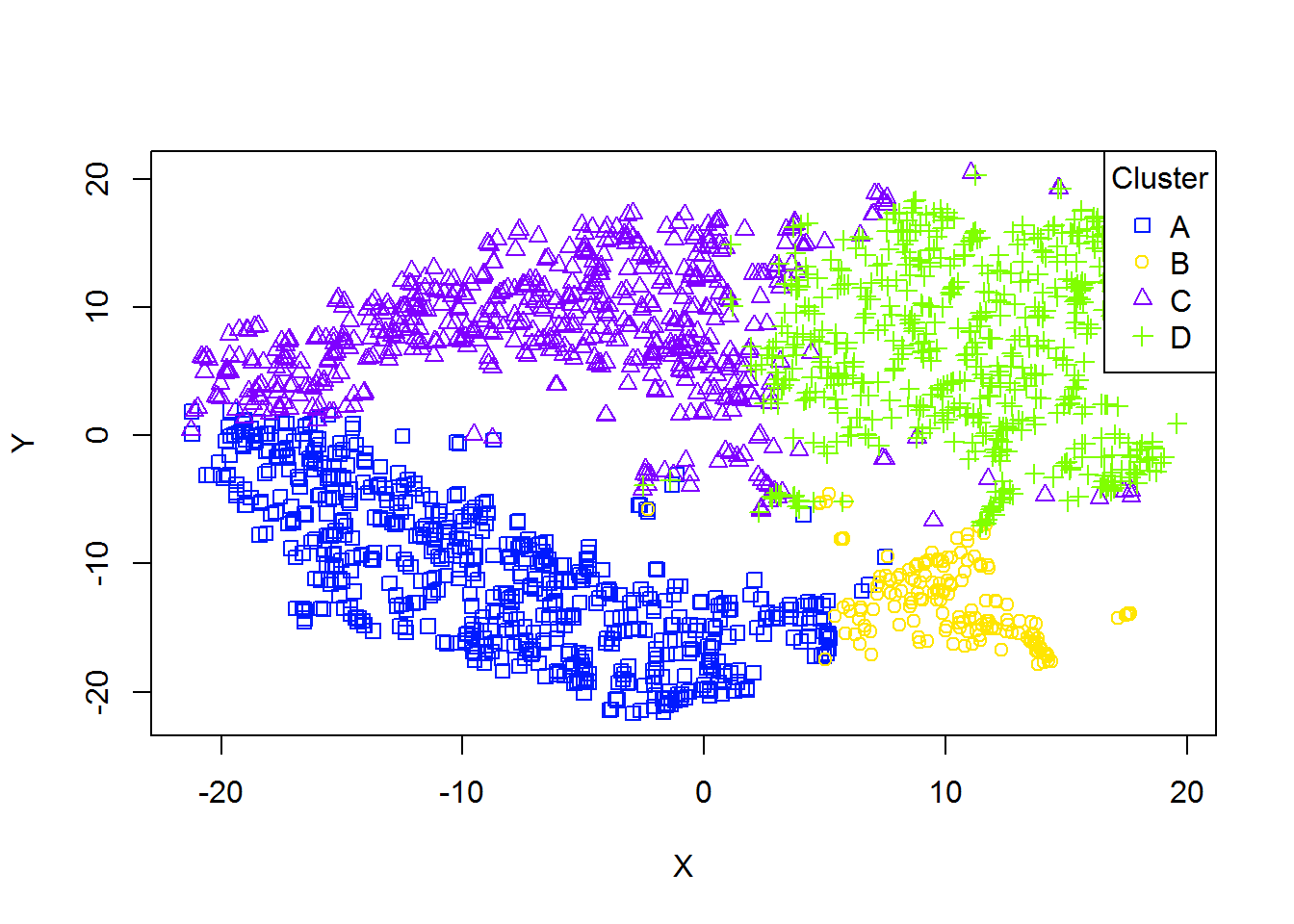
4. K-means clustering
 input_nGenesKNN <- 2000	#Number of genes fro k-Means
 input_nClusters <- 4	#Number of clusters
 maxGeneClustering = 12000
 input_kmeansNormalization <- 'geneMean'	#Normalization
 input_KmeansReRun <- 0	#Random seed

 distributionSD()  #Distribution of standard deviations
KmeansNclusters() #Number of clusters
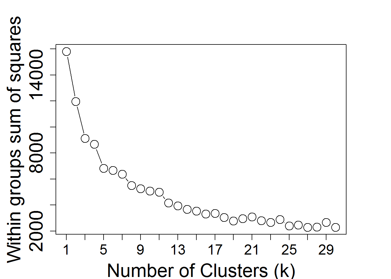
 Kmeans.out = Kmeans()   #Running K-means
 KmeansHeatmap()   #Heatmap for k-Means
 #Read gene sets for enrichment analysis
 sqlite  <- dbDriver('SQLite')
 input_selectGO3 <- 'GOBP'	#Gene set category
 input_minSetSize <- 15	#Min gene set size
 input_maxSetSize <- 2000	#Max gene set size
 GeneSets.out <-readGeneSets( geneSetFile,
    convertedData.out, input_selectGO3,input_selectOrg,
    c(input_minSetSize, input_maxSetSize)  )
 # Alternatively, users can use their own GMT files by
 #GeneSets.out <- readGMTRobust('somefile.GMT')
 results <- KmeansGO()  #Enrichment analysis for k-Means clusters
 results$adj.Pval <- format( results$adj.Pval,digits=3 )
 kable( results, row.names=FALSE)
| Cluster | adj.Pval | Genes | Pathways |
|---|---|---|---|
| A | 2.69e-144 | 121 | RNA processing |
| 1.99e-140 | 106 | Ribonucleoprotein complex biogenesis | |
| 2.29e-134 | 103 | NcRNA metabolic process | |
| 3.50e-117 | 84 | Ribosome biogenesis | |
| 6.34e-115 | 84 | NcRNA processing | |
| 3.48e-107 | 144 | Organonitrogen compound metabolic process | |
| 1.71e-101 | 119 | Organonitrogen compound biosynthetic process | |
| 6.86e-93 | 65 | RRNA processing | |
| 2.89e-92 | 65 | RRNA metabolic process | |
| 5.05e-75 | 74 | Translation | |
| B | 2.08e-25 | 36 | Cellular response to stress |
| 4.56e-23 | 36 | Apoptotic process | |
| 4.56e-23 | 37 | Cell death | |
| 5.85e-23 | 36 | Programmed cell death | |
| 5.85e-23 | 25 | Apoptotic signaling pathway | |
| 1.23e-20 | 24 | Positive regulation of cell death | |
| 1.44e-20 | 23 | Cellular response to DNA damage stimulus | |
| 3.58e-19 | 18 | Intrinsic apoptotic signaling pathway | |
| 1.01e-18 | 22 | Positive regulation of programmed cell death | |
| 1.18e-18 | 14 | Intrinsic apoptotic signaling pathway in response to DNA damage | |
| C | 2.39e-63 | 115 | Immune system process |
| 8.23e-45 | 86 | Positive regulation of response to stimulus | |
| 1.18e-44 | 76 | Immune response | |
| 1.51e-42 | 81 | Establishment of protein localization | |
| 7.23e-42 | 76 | Macromolecular complex assembly | |
| 2.29e-40 | 69 | Regulation of immune system process | |
| 2.29e-40 | 69 | Protein complex assembly | |
| 2.29e-40 | 75 | Protein transport | |
| 2.29e-40 | 69 | Protein complex biogenesis | |
| 2.29e-40 | 72 | Protein complex subunit organization | |
| D | 9.62e-94 | 147 | Immune system process |
| 6.16e-55 | 99 | Positive regulation of response to stimulus | |
| 5.38e-52 | 93 | Positive regulation of molecular function | |
| 6.50e-52 | 93 | Protein phosphorylation | |
| 1.86e-51 | 84 | Defense response | |
| 7.25e-51 | 86 | Regulation of intracellular signal transduction | |
| 1.02e-49 | 72 | Cell activation | |
| 2.24e-47 | 88 | Regulation of transport | |
| 1.00e-46 | 95 | Response to external stimulus | |
| 5.13e-46 | 73 | Vesicle-mediated transport |
 input_seedTSNE <- 0	#Random seed for t-SNE
 input_colorGenes <- TRUE	#Color genes in t-SNE plot?
 tSNEgenePlot()  #Plot genes using t-SNE
## Warning: package 'Rtsne' was built under R version 3.5.1
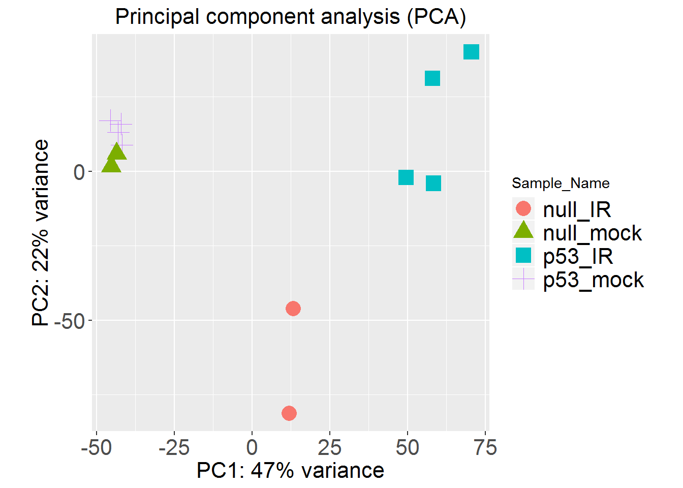
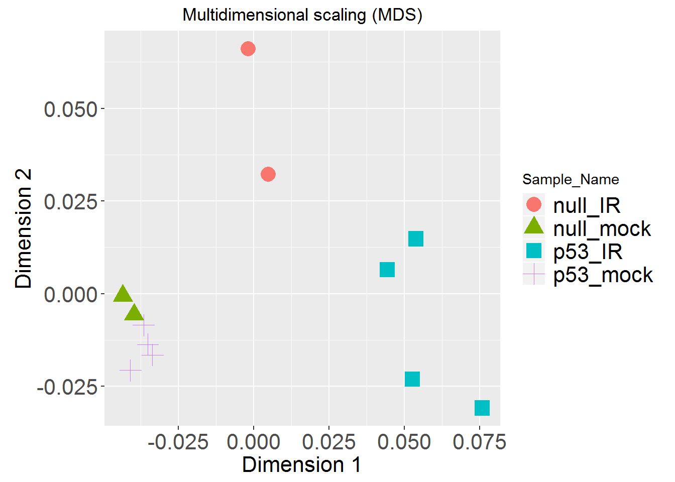
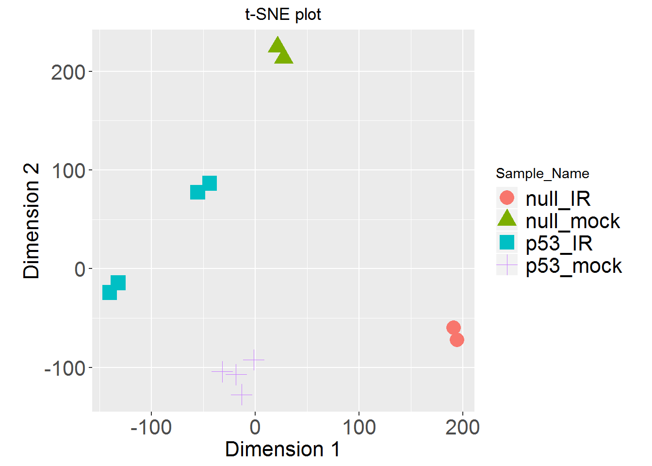
5. PCA and beyond
 input_selectFactors <- 'Sample_Name'	#Factor coded by color
 input_selectFactors2 <- 'Sample_Name'	#Factor coded by shape
 input_tsneSeed2 <- 0	#Random seed for t-SNE
 #PCA, MDS and t-SNE plots
 PCAplot()
MDSplot()
tSNEplot()
 #Read gene sets for pathway analysis using PGSEA on principal components
 input_selectGO6 <- 'GOBP'
 GeneSets.out <-readGeneSets( geneSetFile,
    convertedData.out, input_selectGO6,input_selectOrg,
    c(input_minSetSize, input_maxSetSize)  )
 PCApathway() # Run PGSEA analysis
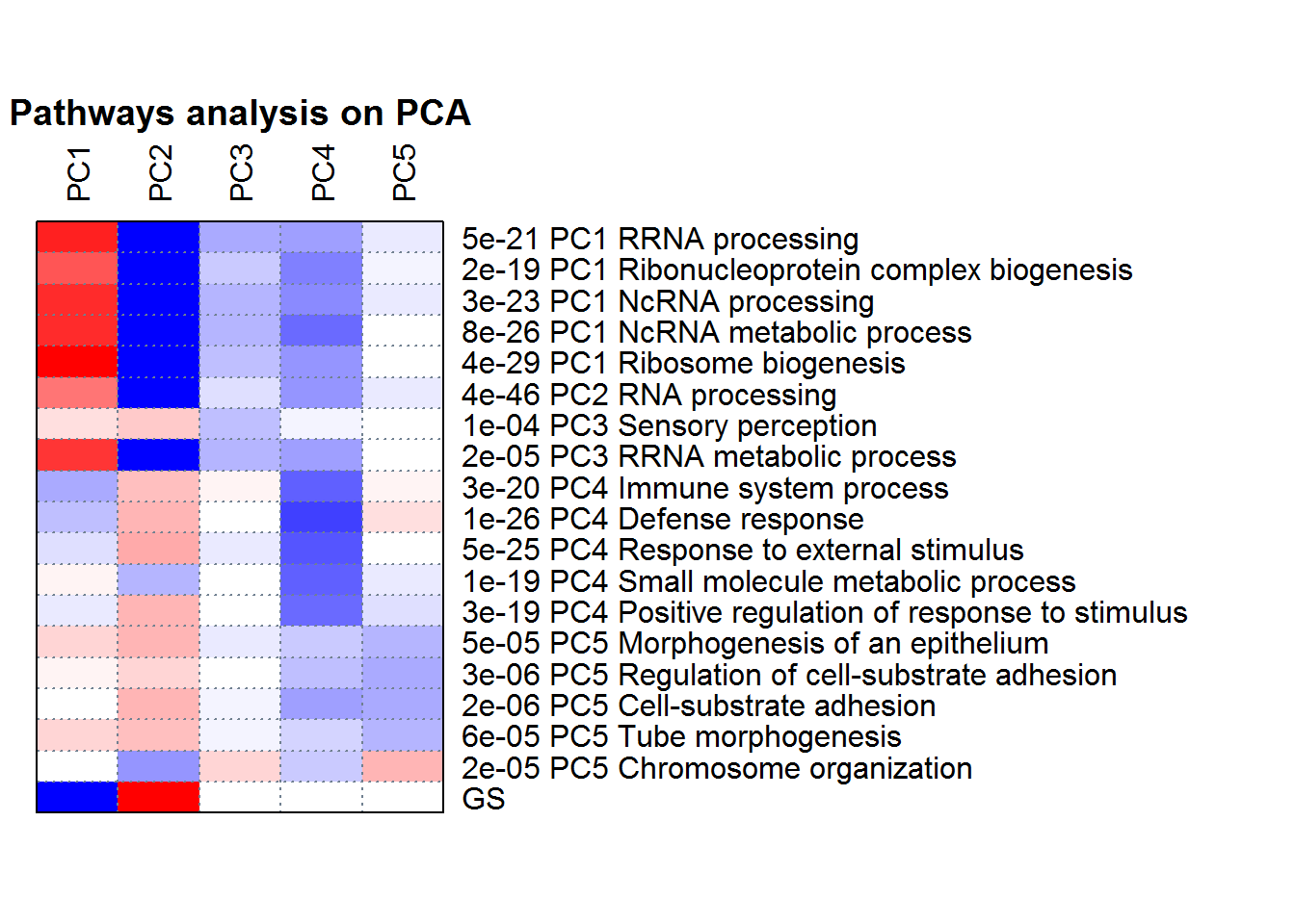
cat( PCA2factor() ) #The correlation between PCs with factors
##
##  Correlation between Principal Components (PCs) with factors
## PC1 is correlated with Treatment (p=6.56e-05).
6. Differentially Expressed Genes (DEG1)
 input_CountsDEGMethod <- 3	#DESeq2= 3,limma-voom=2,limma-trend=1
 input_limmaPval <- 0.1	#FDR cutoff
 input_limmaFC <- 2	#Fold-change cutoff
 input_selectModelComprions <- c('p53: wt vs. null','Treatment: IR vs. mock')	#Selected comparisons
 input_selectFactorsModel <- c('p53','Treatment')	#Selected comparisons
 input_selectInteractions <- 'p53:Treatment'	#Selected comparisons
 input_selectBlockFactorsModel <- NULL 	#Selected comparisons
 factorReferenceLevels.out <- c('p53:null','Treatment:mock')

 limma.out <- limma()
 DEG.data.out <- DEG.data()
 limma.out$comparisons
## [1] "wt-null"               "IR-mock"               "I:p53_wt.Treatment_IR"
## [4] "wt-null_for_IR"        "IR-mock_for_wt"
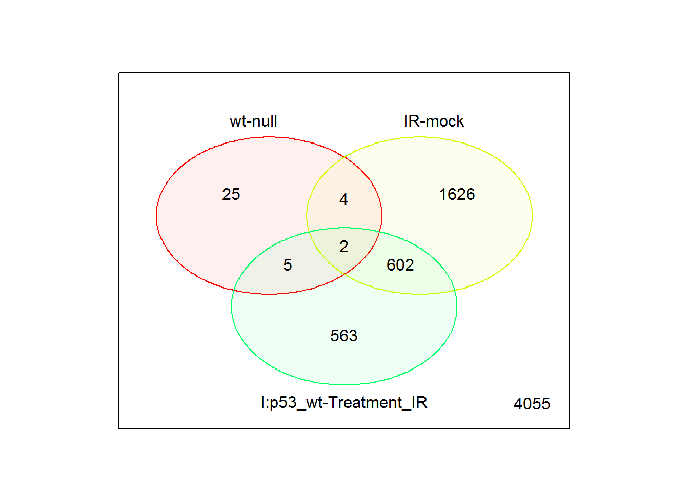
 input_selectComparisonsVenn = limma.out$comparisons[1:3] # use first three comparisons
 input_UpDownRegulated <- FALSE	#Split up and down regulated genes
 vennPlot() # Venn diagram
sigGeneStats() # number of DEGs as figure
sigGeneStatsTable() # number of DEGs as table
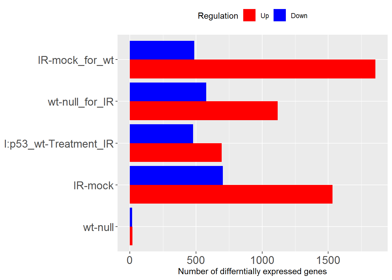
##                                 Comparisons   Up Down
## wt-null                             wt-null   20   16
## IR-mock                             IR-mock 1532  702
## I:p53_wt-Treatment_IR I:p53_wt-Treatment_IR  694  478
## wt-null_for_IR               wt-null_for_IR 1118  577
## IR-mock_for_wt               IR-mock_for_wt 1856  487
7. Differentially Expressed Genes (DEG1)
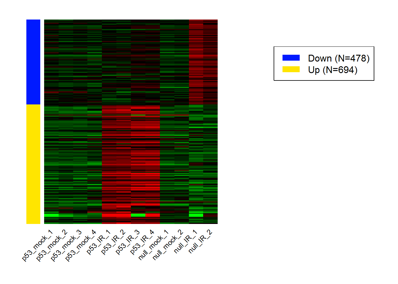
 input_selectContrast <- 'I:p53_wt.Treatment_IR'	#Selected comparisons
 selectedHeatmap.data.out <- selectedHeatmap.data()
 selectedHeatmap()   # heatmap for DEGs in selected comparison
 # Save gene lists and data into files
 write.csv( selectedHeatmap.data()$genes, 'heatmap.data.csv')
 write.csv(DEG.data(),'DEG.data.csv' )
 write(AllGeneListsGMT() ,'AllGeneListsGMT.gmt')
input_selectGO2 <- 'GSKB.TF.Target' #Gene set category
geneListData.out <- geneListData()
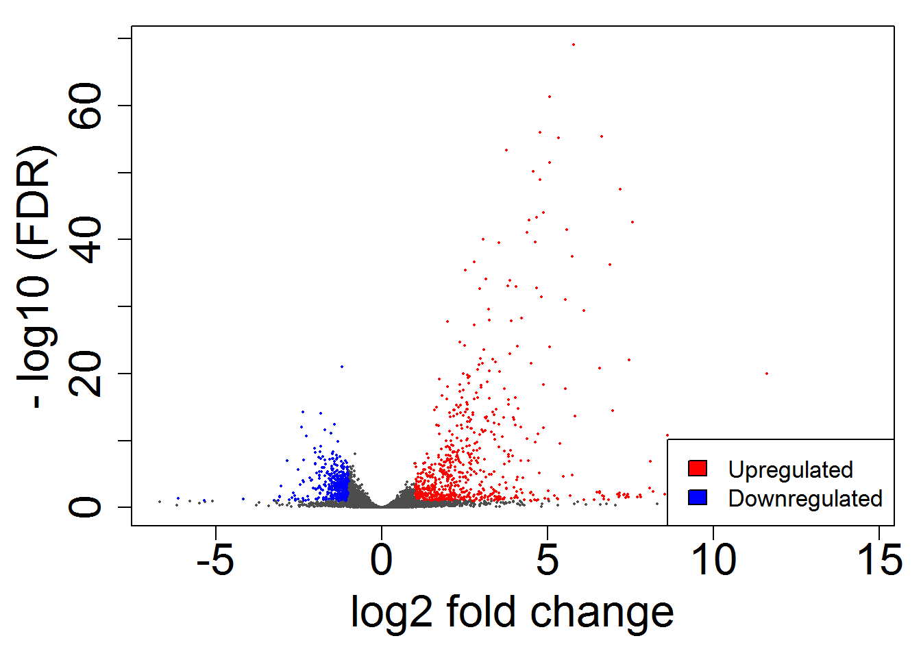
volcanoPlot()
# scatterPlot()
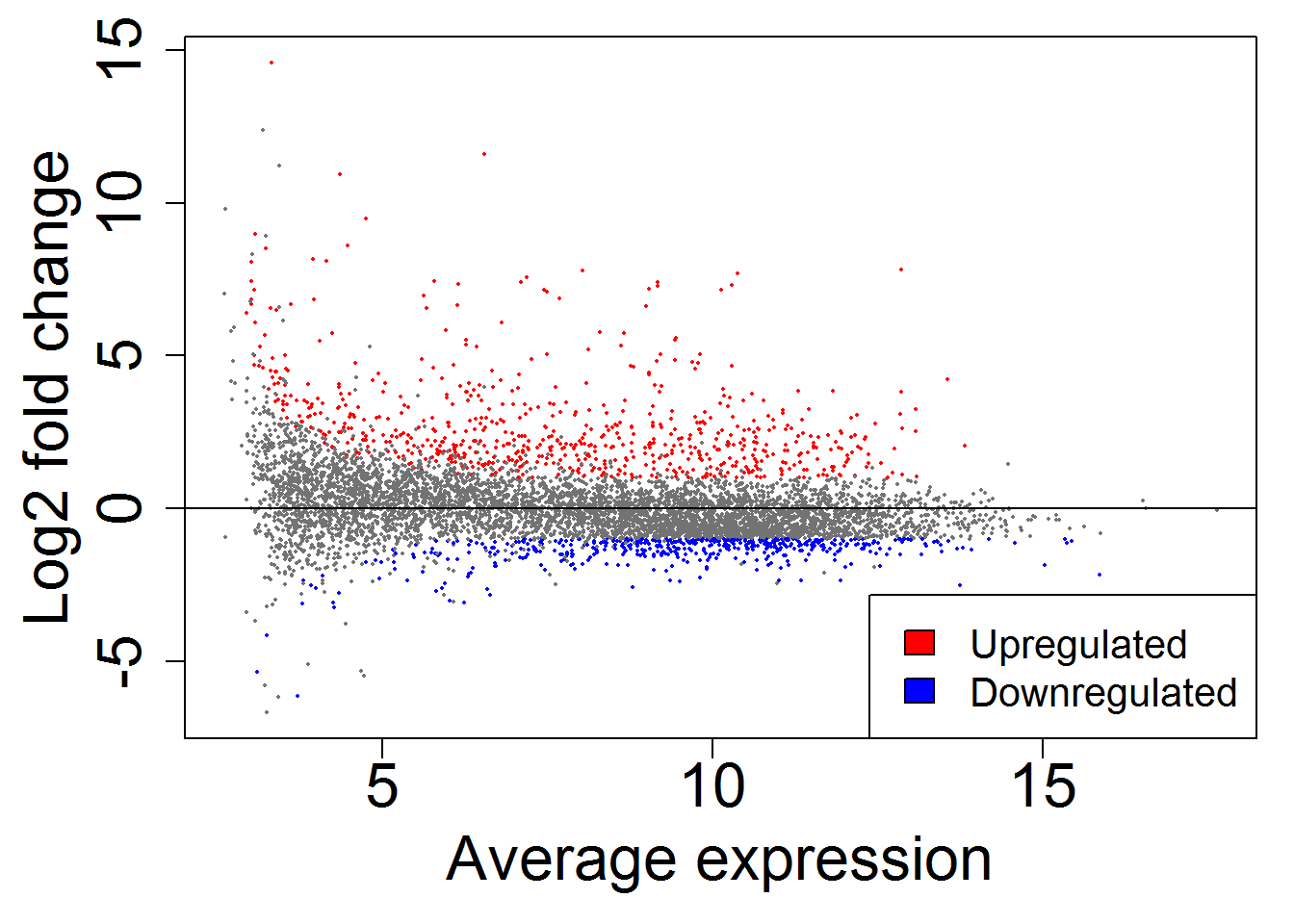
MAplot()
  geneListGOTable.out <- geneListGOTable()
 # Read pathway data again
 GeneSets.out <-readGeneSets( geneSetFile,
    convertedData.out, input_selectGO2,input_selectOrg,
    c(input_minSetSize, input_maxSetSize)  )
 input_removeRedudantSets <- TRUE	#Remove highly redundant gene sets?
 results <- geneListGO()  #Enrichment analysis for k-Means clusters
 results$adj.Pval <- format( results$adj.Pval,digits=3 )
 kable( results, row.names=FALSE)
| Direction | adj.Pval | nGenes | Pathways |
|---|---|---|---|
| Down regulated | 3.3e-61 | 95 | Organonitrogen compound metabolic process |
| 4.8e-53 | 84 | Small molecule metabolic process | |
| 1.2e-51 | 75 | Cell cycle | |
| 1.4e-48 | 62 | DNA metabolic process | |
| 3.4e-45 | 67 | Organonitrogen compound biosynthetic process | |
| 6.7e-45 | 61 | Cell cycle process | |
| 7.2e-43 | 71 | Macromolecular complex assembly | |
| 2.5e-40 | 68 | Cellular response to stress | |
| 3.0e-40 | 52 | Mitotic cell cycle | |
| 7.6e-39 | 49 | Mitotic cell cycle process | |
| Up regulated | 6.0e-41 | 82 | Tissue development |
| 6.8e-39 | 79 | Regulation of transcription from RNA polymerase II promoter | |
| 6.8e-39 | 80 | Transcription from RNA polymerase II promoter | |
| 6.8e-39 | 85 | Apoptotic process | |
| 6.8e-39 | 84 | Cell development | |
| 1.5e-38 | 85 | Programmed cell death | |
| 7.7e-38 | 86 | Cell death | |
| 2.1e-37 | 78 | Positive regulation of nitrogen compound metabolic process | |
| 5.5e-36 | 74 | Positive regulation of nucleobase-containing compound metabolic process | |
| 1.3e-35 | 86 | Cellular response to organic substance |
STRING-db API access. We need to find the taxonomy id of your species, this used by STRING. First we try to guess the ID based on iDEP’s database. Users can also skip this step and assign NCBI taxonomy id directly by findTaxonomyID.out = 10090 # mouse 10090, human 9606 etc.
 STRING10_species = read.csv(STRING10_speciesFile)
 ix = grep('Mus musculus', STRING10_species$official_name )
 findTaxonomyID.out <- STRING10_species[ix,1] # find taxonomyID
 findTaxonomyID.out
## [1] 10090
Enrichment analysis using STRING
STRINGdb_geneList.out <- STRINGdb_geneList() #convert gene lists
## Warning: we couldn't map to STRING 8% of your identifiers
 input_STRINGdbGO <- 'Process'	#'Process', 'Component', 'Function', 'KEGG', 'Pfam', 'InterPro'
 results <- stringDB_GO_enrichmentData()  # enrichment using STRING
 results$adj.Pval <- format( results$adj.Pval,digits=3 )
 kable( results, row.names=FALSE)
| Direction | adj.Pval | nGenes | Pathways |
|---|---|---|---|
| Up regulated | 4.5e-11 | 66 | intracellular signal transduction |
| 2.6e-10 | 51 | apoptotic process | |
| 4.5e-10 | 51 | programmed cell death | |
| 9.8e-10 | 51 | cell death | |
| 9.8e-10 | 51 | death | |
| 2.2e-09 | 71 | tissue development | |
| 4.1e-09 | 26 | apoptotic signaling pathway | |
| 5.2e-09 | 20 | intrinsic apoptotic signaling pathway | |
| 9.7e-09 | 15 | intrinsic apoptotic signaling pathway in response to DNA damage | |
| 1.7e-08 | 58 | regulation of apoptotic process | |
| 3.2e-08 | 65 | cell development | |
| 3.7e-08 | 62 | positive regulation of molecular function | |
| 5.2e-08 | 47 | negative regulation of signal transduction | |
| 5.2e-08 | 62 | cell surface receptor signaling pathway | |
| 5.2e-08 | 57 | regulation of programmed cell death | |
| Down regulated | 2.2e-15 | 60 | cell cycle |
| 5.2e-15 | 25 | protein folding | |
| 3.1e-14 | 65 | small molecule metabolic process | |
| 3.1e-14 | 33 | small molecule biosynthetic process | |
| 1.1e-13 | 53 | single-organism biosynthetic process | |
| 3.4e-13 | 61 | organonitrogen compound metabolic process | |
| 5.2e-13 | 46 | organonitrogen compound biosynthetic process | |
| 2.4e-12 | 38 | mitotic cell cycle | |
| 2.4e-12 | 46 | cell cycle process | |
| 3.1e-12 | 37 | mitotic cell cycle process | |
| 7.6e-12 | 30 | ncRNA metabolic process | |
| 2.8e-11 | 24 | organic acid biosynthetic process | |
| 2.8e-11 | 24 | carboxylic acid biosynthetic process | |
| 5.0e-11 | 33 | cell division | |
| 8.6e-11 | 37 | DNA metabolic process |
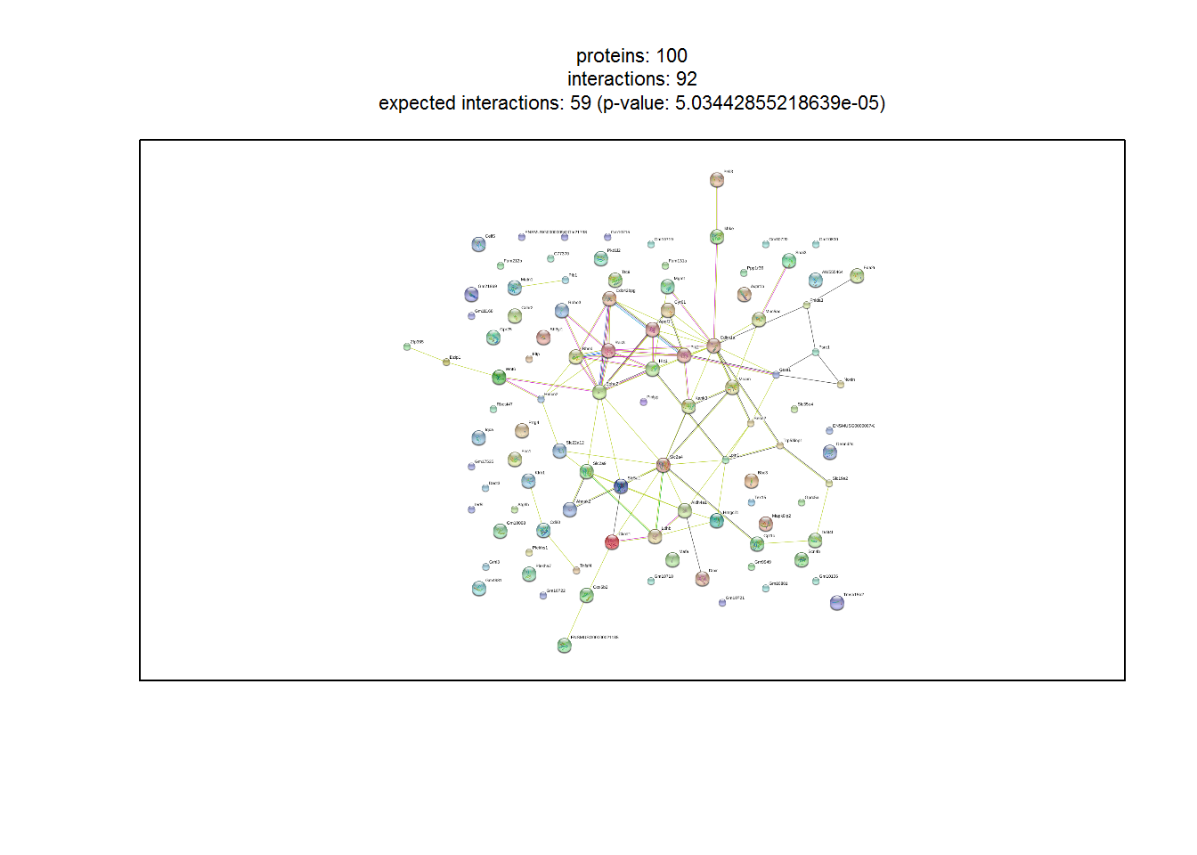
PPI network retrieval and analysis
 input_nGenesPPI <- 100	#Number of top genes for PPI retrieval and analysis
 stringDB_network1(1) #Show PPI network
 Generating interactive PPI
write(stringDB_network_link(), 'PPI_results.html') # write results to html file
## Warning: we couldn't map to STRING 8% of your identifiers
browseURL('PPI_results.html') # open in browser
8. Pathway analysis
 input_selectContrast1 <- 'I:p53_wt.Treatment_IR'	#select Comparison
 #input_selectContrast1 = limma.out$comparisons[3] # manually set
 input_selectGO <- 'KEGG'	#Gene set category
 #input_selectGO='custom' # if custom gmt file
 input_minSetSize <- 15	#Min size for gene set
 input_maxSetSize <- 2000	#Max size for gene set
 # Read pathway data again
 GeneSets.out <-readGeneSets( geneSetFile,
    convertedData.out, input_selectGO,input_selectOrg,
    c(input_minSetSize, input_maxSetSize)  )
 input_pathwayPvalCutoff <- 0.2	#FDR cutoff
 input_nPathwayShow <- 30	#Top pathways to show
 input_absoluteFold <- FALSE	#Use absolute values of fold-change?
 input_GenePvalCutoff <- 1	#FDR to remove genes

 input_pathwayMethod = 1  # 1  GAGE
 gagePathwayData.out <- gagePathwayData()  # pathway analysis using GAGE

 results <- gagePathwayData.out  #Enrichment analysis for k-Means clusters
 results$adj.Pval <- format( results$adj.Pval,digits=3 )
 kable( results, row.names=FALSE)
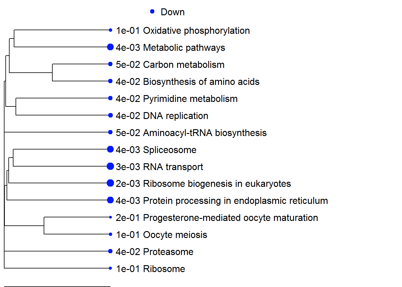
| Direction | GAGE analysis: I:p53_wt.Treatment_IR | statistic | Genes | adj.Pval |
|---|---|---|---|---|
| Down | Ribosome biogenesis in eukaryotes | -4.6634 | 40 | 2.3e-03 |
| RNA transport | -4.2098 | 62 | 2.9e-03 | |
| Spliceosome | -4.0557 | 39 | 4.5e-03 | |
| Protein processing in endoplasmic reticulum | -3.9119 | 54 | 4.5e-03 | |
| Metabolic pathways | -3.7276 | 449 | 4.5e-03 | |
| DNA replication | -3.4728 | 20 | 3.5e-02 | |
| Proteasome | -3.221 | 23 | 4.1e-02 | |
| Aminoacyl-tRNA biosynthesis | -3.2197 | 17 | 5.0e-02 | |
| Pyrimidine metabolism | -3.1178 | 50 | 4.0e-02 | |
| Biosynthesis of amino acids | -3.1022 | 32 | 4.1e-02 | |
| Carbon metabolism | -2.9154 | 47 | 5.0e-02 | |
| Oxidative phosphorylation | -2.5729 | 46 | 1.1e-01 | |
| Ribosome | -2.5555 | 28 | 1.2e-01 | |
| Oocyte meiosis | -2.5519 | 39 | 1.1e-01 | |
| Progesterone-mediated oocyte maturation | -2.2879 | 27 | 2.0e-01 |
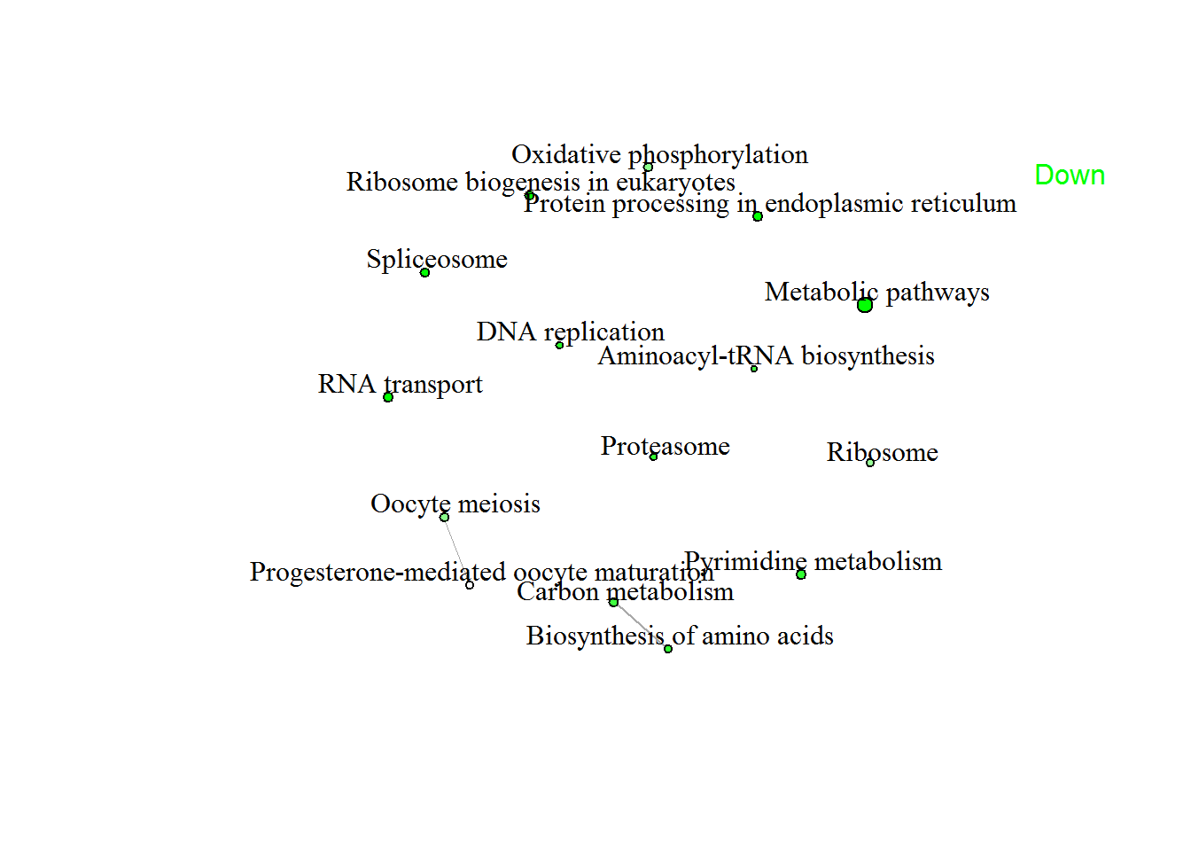
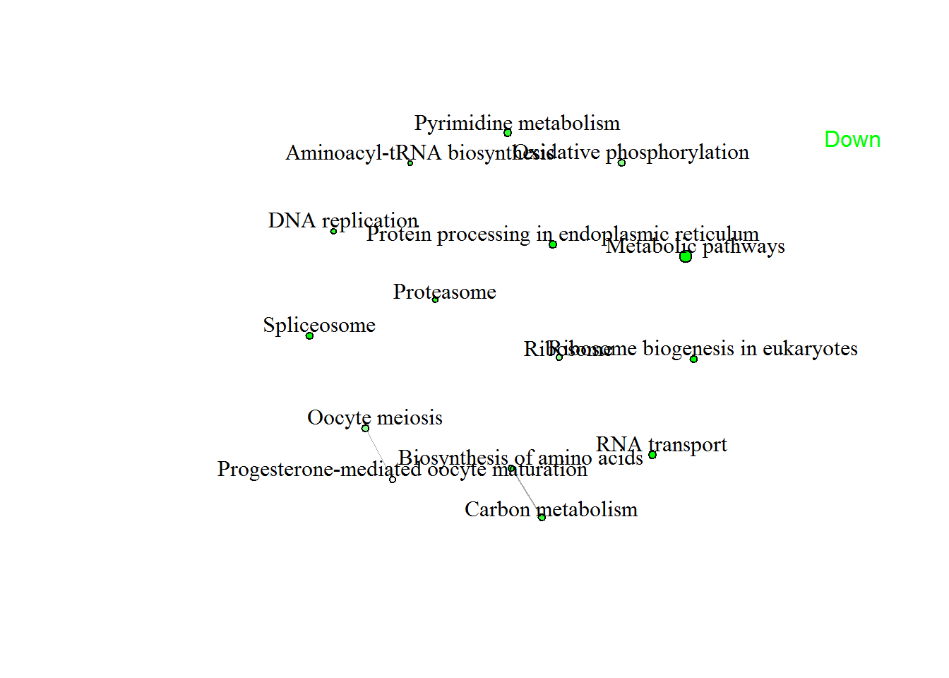
 pathwayListData.out = pathwayListData()
 enrichmentPlot(pathwayListData.out, 25  )
## Warning: package 'dendextend' was built under R version 3.5.1

enrichmentNetwork(pathwayListData.out )
## Warning: package 'igraph' was built under R version 3.5.1
# enrichmentNetworkPlotly(pathwayListData.out)
 input_pathwayMethod = 3  # 1  fgsea
 fgseaPathwayData.out <- fgseaPathwayData() #Pathway analysis using fgsea
 results <- fgseaPathwayData.out  #Enrichment analysis for k-Means clusters
 results$adj.Pval <- format( results$adj.Pval,digits=3 )
 kable( results, row.names=FALSE)
  pathwayListData.out = pathwayListData()
 enrichmentPlot(pathwayListData.out, 25  )
enrichmentNetwork(pathwayListData.out )
# enrichmentNetworkPlotly(pathwayListData.out)
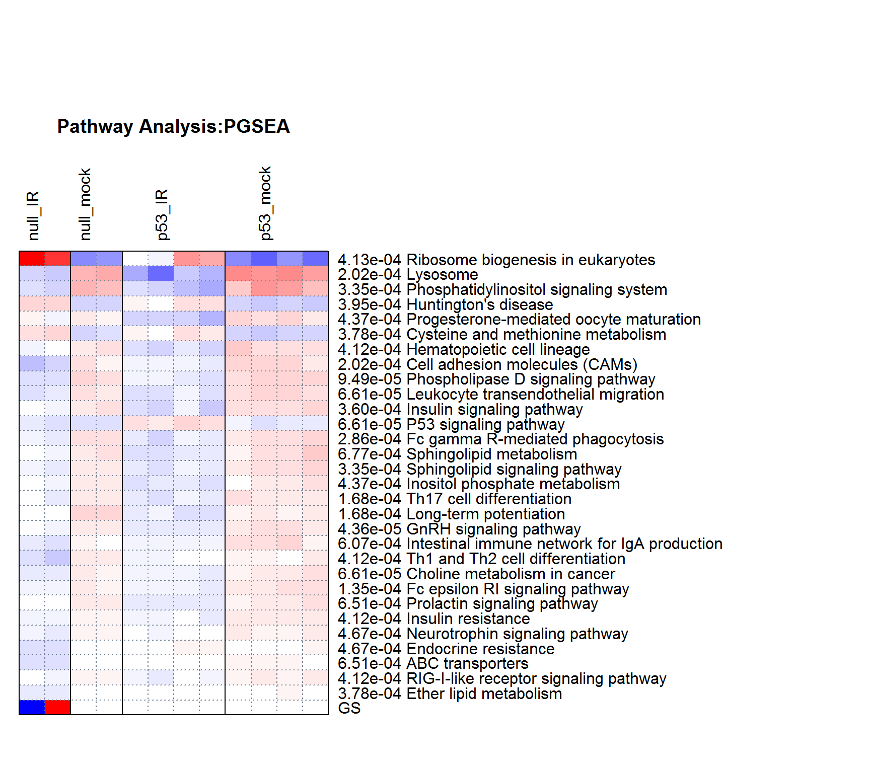
PGSEAplot() # pathway analysis using PGSEA
##
## Computing P values using ANOVA
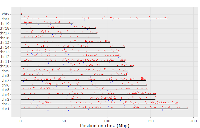
9. Chromosome
 input_selectContrast2 <- 'IR-mock_for_wt'	#select Comparison
 #input_selectContrast2 = limma.out$comparisons[3] # manually set
 input_limmaPvalViz <- 0.1	#FDR to filter genes
 input_limmaFCViz <- 2	#FDR to filter genes
# genomePlotly() # shows fold-changes on the genome
10. Biclustering
 input_nGenesBiclust <- 1000	#Top genes for biclustering
 input_biclustMethod <- 'BCCC()'	#Method: 'BCCC', 'QUBIC', 'runibic' ...
 biclustering.out = biclustering()  # run analysis
## Warning: package 'biclust' was built under R version 3.5.1
 input_selectBicluster <- 1	#select a cluster
 biclustHeatmap()   # heatmap for selected cluster
 input_selectGO4 <- 'GOBP'	#Gene set category
 # Read pathway data again
 GeneSets.out <-readGeneSets( geneSetFile,
    convertedData.out, input_selectGO4,input_selectOrg,
    c(input_minSetSize, input_maxSetSize)  )
 results <- geneListBclustGO()  #Enrichment analysis for k-Means clusters
 results$adj.Pval <- format( results$adj.Pval,digits=3 )
 kable( results, row.names=FALSE)
| adj.Pval | Genes | Pathways |
|---|---|---|
| 3.1e-124 | 207 | Immune system process |
| 1.5e-89 | 157 | Organonitrogen compound metabolic process |
| 4.7e-86 | 148 | Positive regulation of molecular function |
| 5.4e-86 | 155 | Cell death |
| 2.0e-83 | 139 | Homeostatic process |
| 3.2e-81 | 136 | Macromolecular complex assembly |
| 3.5e-80 | 146 | Programmed cell death |
| 2.9e-79 | 144 | Apoptotic process |
| 1.1e-75 | 132 | Regulation of cell death |
| 2.2e-75 | 117 | Cell-cell adhesion |
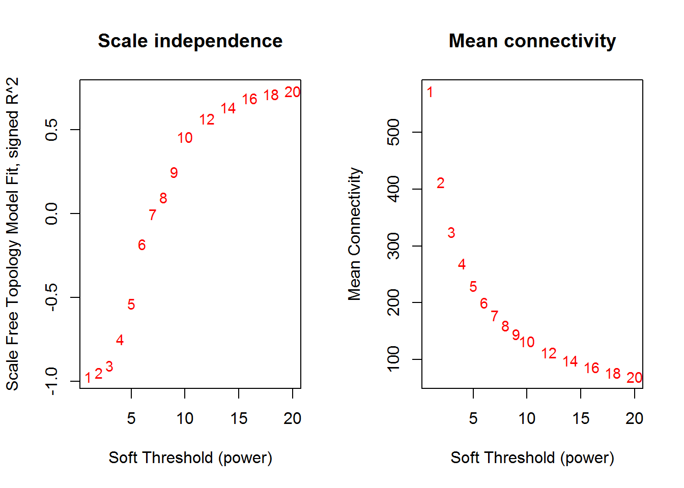
11. Co-expression network
 input_mySoftPower <- 5	#SoftPower to cutoff
 input_nGenesNetwork <- 1000	#Number of top genes
 input_minModuleSize <- 20	#Module size minimum
 wgcna.out = wgcna()   # run WGCNA
## ==========================================================================
## *
## *  Package WGCNA 1.63 loaded.
## *
## *    Important note: It appears that your system supports multi-threading,
## *    but it is not enabled within WGCNA in R.
## *    To allow multi-threading within WGCNA with all available cores, use
## *
## *          allowWGCNAThreads()
## *
## *    within R. Use disableWGCNAThreads() to disable threading if necessary.
## *    Alternatively, set the following environment variable on your system:
## *
## *          ALLOW_WGCNA_THREADS=<number_of_processors>
## *
## *    for example
## *
## *          ALLOW_WGCNA_THREADS=8
## *
## *    To set the environment variable in linux bash shell, type
## *
## *           export ALLOW_WGCNA_THREADS=8
## *
## *     before running R. Other operating systems or shells will
## *     have a similar command to achieve the same aim.
## *
## ==========================================================================
##
##
##    Power SFT.R.sq   slope truncated.R.sq mean.k. median.k. max.k.
## 1      1   0.9720  2.7600          0.966   572.0     612.0    711
## 2      2   0.9490  1.2200          0.956   412.0     449.0    578
## 3      3   0.9050  0.7070          0.923   325.0     353.0    495
## 4      4   0.7480  0.4190          0.797   269.0     287.0    439
## 5      5   0.5350  0.2490          0.615   230.0     239.0    398
## 6      6   0.1820  0.1090          0.255   200.0     204.0    367
## 7      7   0.0040  0.0131          0.185   178.0     175.0    342
## 8      8   0.0965 -0.0738          0.144   160.0     152.0    321
## 9      9   0.2500 -0.1240          0.238   145.0     133.0    303
## 10    10   0.4570 -0.1930          0.431   132.0     118.0    287
## 11    12   0.5670 -0.2940          0.514   113.0      98.9    263
## 12    14   0.6340 -0.3830          0.587    97.8      84.7    243
## 13    16   0.6890 -0.4420          0.655    86.2      73.5    227
## 14    18   0.7120 -0.4930          0.673    76.9      63.8    213
## 15    20   0.7290 -0.5420          0.683    69.3      55.7    201
## TOM calculation: adjacency..
## ..will not use multithreading.
##  Fraction of slow calculations: 0.000000
## ..connectivity..
## ..matrix multiplication (system BLAS)..
## ..normalization..
## ..done.
softPower() # soft power curve
modulePlot() # plot modules
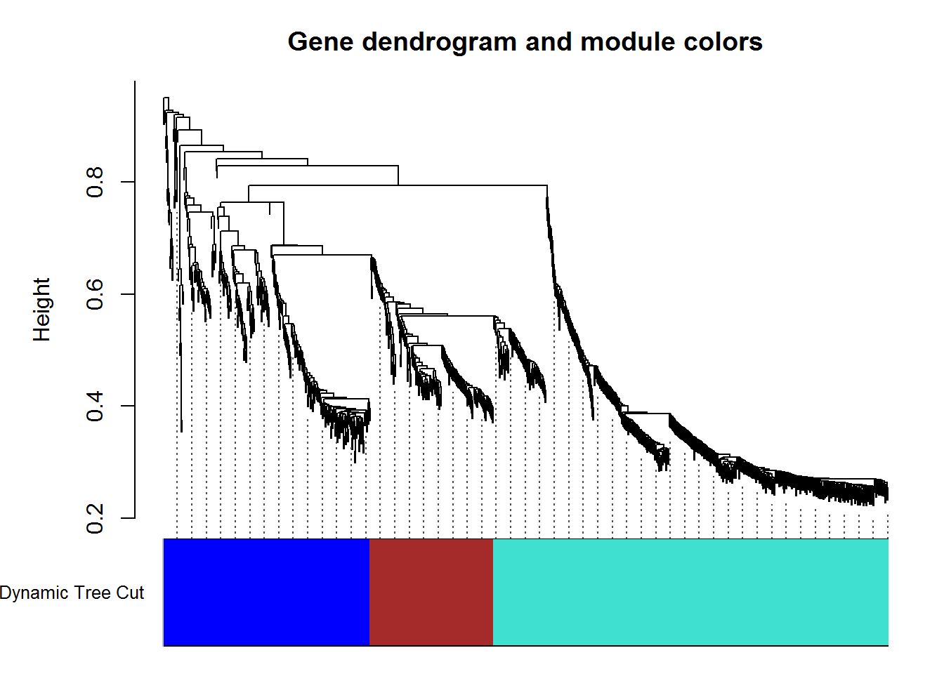
listWGCNA.Modules.out = listWGCNA.Modules() #modules
input_selectGO5 <- 'GOBP' #Gene set category
# Read pathway data again
GeneSets.out <-readGeneSets( geneSetFile,
convertedData.out, input_selectGO5,input_selectOrg,
c(input_minSetSize, input_maxSetSize) )
input_selectWGCNA.Module <- '1. turquoise (495 genes)' #Select a module
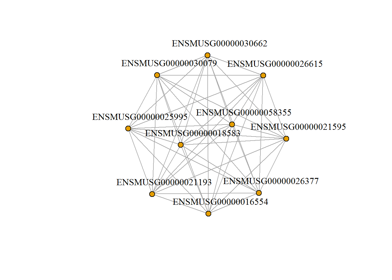
input_topGenesNetwork <- 10 #SoftPower to cutoff
input_edgeThreshold <- 0.4 #Number of top genes
moduleNetwork() # show network of top genes in selected module
##  softConnectivity: FYI: connecitivty of genes with less than 4 valid samples will be returned as NA.
##  ..calculating connectivities..
 input_removeRedudantSets <- TRUE	#Remove redundant gene sets
 results <- networkModuleGO()  #Enrichment analysis of selected module
 results$adj.Pval <- format( results$adj.Pval,digits=3 )
 kable( results, row.names=FALSE)
| adj.Pval | Genes | Pathways |
|---|---|---|
| 6.2e-68 | 106 | Organonitrogen compound metabolic process |
| 3.0e-62 | 61 | Ribonucleoprotein complex biogenesis |
| 6.9e-62 | 68 | RNA processing |
| 4.0e-61 | 84 | Organonitrogen compound biosynthetic process |
| 2.4e-56 | 57 | NcRNA metabolic process |
| 4.2e-53 | 101 | Immune system process |
| 2.0e-49 | 81 | Macromolecular complex assembly |
| 3.0e-48 | 46 | Ribosome biogenesis |
| 3.4e-48 | 84 | Establishment of protein localization |
| 4.7e-48 | 63 | Cellular amide metabolic process |