Update. 11/13/17 Thanks to Mike Love for pointing out an error. This is just my understanding. There maybe other errors.
To allow complex study designs in iDEP(http://ge-lab.org/idep/), I tried to understand how factoral models are built and the desired results are extracted from DESeq2. The following is based on the help document from the resutls( ) function in DESeq2, plus some of Mike Love’s answers to questions from users.
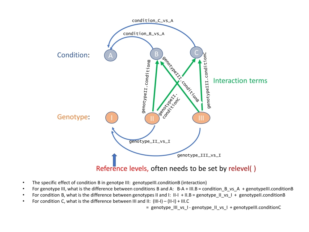
An important point I want to make is the interpretation of results is tricky when the study design involve multiple factors. See figure above for an example involving 3 genotypes under 3 conditions. Similar to regression analysis in R, the reference levels for categorical factors forms the foundation of our intereptation. Yet, by default, they are determined alphabetically.
Before runing DESeq2, it is essential to choose appropriate reference levels for each factors. This can be done by the relevel( ) function in R. Reference level is the baseline level of a factor that forms the basis of meaningful comparisons. In a wildtype vs. mutant experiment, “wild-type” is the reference level. In treated vs. untreated, the reference level is obviously untreated. More details in Exmple 3.
iDEP provides a GUI to DESeq2 for most experimental desings. It also provides convienent interface for exploratory data anlysis and pathway analysis. Try it at http://ge-lab.org/idep/
Example 1: two-group comparison
First make some example data.
library(DESeq2)
dds <- makeExampleDESeqDataSet(n=10000,m=6)
assay(dds)[ 1:10,]
##        sample1 sample2 sample3 sample4 sample5 sample6
## gene1        6       4      11       1       2      13
## gene2        9      12      23      13      14      28
## gene3       58     121     173     178     118      97
## gene4        0       4       0       3       8       3
## gene5       27       3       6       9       8      12
## gene6       48       8      35      38      21      13
## gene7       36      50      61      52      44      22
## gene8        6       8      16      14      18      19
## gene9      214     266     419     198     157     166
## gene10      20      12      16      12      16       2
This is a very simple experiment design with two conditions.
colData(dds)
## DataFrame with 6 rows and 1 column
##         condition
##          <factor>
## sample1         A
## sample2         A
## sample3         A
## sample4         B
## sample5         B
## sample6         B
dds <- DESeq(dds)
resultsNames(dds)
## [1] "Intercept" "condition_B_vs_A"
This shows the results available. Note that by default, R will choose a reference level for factors based on alphabetical order. Here A is the referece level. Fold change is defined as B compaired with A. To change reference levels, try the relevel( ) function.
res <- results(dds, contrast=c("condition","B","A"))
res <- res[order(res$padj),]
library(knitr)
kable(res[1:5,-(3:4)])
| baseMean | log2FoldChange | pvalue | padj | |
|---|---|---|---|---|
| gene9056 | 360.168909 | -2.045379 | 0.0000000 | 0.0001372 |
| gene3087 | 43.897516 | -2.203303 | 0.0000173 | 0.0857004 |
| gene3763 | 72.409877 | -1.834787 | 0.0000433 | 0.1434364 |
| gene2054 | 322.494963 | 1.537408 | 0.0000682 | 0.1692730 |
| gene4617 | 6.227415 | 6.125238 | 0.0002015 | 0.4001027 |
If we want to use B as control and define fold change using B as baseline. Then we can do this:
res <- results(dds, contrast=c("condition","A","B"))
ix = which.min(res$padj)
res <- res[order(res$padj),]
kable(res[1:5,-(3:4)])
| baseMean | log2FoldChange | pvalue | padj | |
|---|---|---|---|---|
| gene9056 | 360.168909 | 2.045379 | 0.0000000 | 0.0001372 |
| gene3087 | 43.897516 | 2.203303 | 0.0000173 | 0.0857004 |
| gene3763 | 72.409877 | 1.834787 | 0.0000433 | 0.1434364 |
| gene2054 | 322.494963 | -1.537408 | 0.0000682 | 0.1692730 |
| gene4617 | 6.227415 | -6.125238 | 0.0002015 | 0.4001027 |
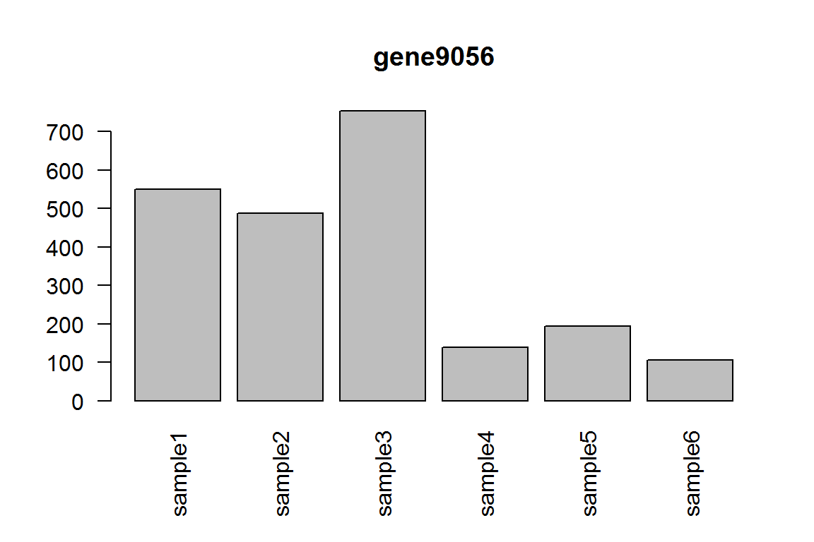
As you can see, the fold-change are completely opposite direction. Here we show the most significant gene.
barplot(assay(dds)[ix,],las=2, main=rownames(dds)[ ix ] )
#Example 2: Multiple groups Suppose we have three groups A, B, and C.
dds <- makeExampleDESeqDataSet(n=100,m=6)
dds$condition <- factor( c( "A","A","B","B","C","C") )
dds <- DESeq(dds)
res = results(dds, contrast=c("condition","C","A"))
res <- res[order(res$padj),]
kable(res[1:5,-(3:4)])
| baseMean | log2FoldChange | pvalue | padj | |
|---|---|---|---|---|
| gene2 | 3.634986 | -5.101773 | 0.0348679 | 0.5515088 |
| gene20 | 4.678176 | -4.490982 | 0.0445664 | 0.5515088 |
| gene34 | 56.068672 | -1.462155 | 0.0167820 | 0.5515088 |
| gene35 | 537.847175 | -1.177240 | 0.0087913 | 0.5515088 |
| gene41 | 93.967810 | 1.064734 | 0.0412034 | 0.5515088 |
Example 3: two conditions, two genotypes, with an interaction term
Here we have two genotypes, wild-type (WT), and mutant (MU). Two conditions, control (Ctrl) and treated (Trt). We are interested in the responses of both wild-type and mutant to treatment. We are also interested in the differences in response between genotypes, which is captured by the interaction term in linear models.
First, we construct example data. Note that we changed sample names from “sample1” to “Wt_Ctrl_1”, according to the two factors.
dds <- makeExampleDESeqDataSet(n=10000,m=12)
dds$condition <- factor( c( rep("Ctrl",6), rep("Trt",6) ) )
dds$genotype <- factor(rep(rep(c("WT","MU"),each=3),2))
colnames(dds) <- paste(as.character( dds$genotype),as.character( dds$condition),rownames(colData(dds)),  sep="_"  )
colnames(dds) = gsub("sample","",colnames(dds))
kable(assay(dds)[1:5,])
| WT_Ctrl_1 | WT_Ctrl_2 | WT_Ctrl_3 | MU_Ctrl_4 | MU_Ctrl_5 | MU_Ctrl_6 | WT_Trt_7 | WT_Trt_8 | WT_Trt_9 | MU_Trt_10 | MU_Trt_11 | MU_Trt_12 | |
|---|---|---|---|---|---|---|---|---|---|---|---|---|
| gene1 | 81 | 47 | 135 | 72 | 81 | 80 | 76 | 57 | 52 | 49 | 64 | 57 |
| gene2 | 70 | 77 | 94 | 54 | 54 | 36 | 51 | 66 | 57 | 51 | 47 | 67 |
| gene3 | 16 | 37 | 8 | 28 | 4 | 36 | 14 | 10 | 7 | 11 | 40 | 15 |
| gene4 | 2 | 5 | 1 | 3 | 9 | 2 | 1 | 5 | 0 | 0 | 14 | 8 |
| gene5 | 0 | 0 | 1 | 0 | 5 | 0 | 0 | 0 | 0 | 0 | 0 | 0 |
kable( colData(dds))
| condition | genotype | |
|---|---|---|
| WT_Ctrl_1 | Ctrl | WT |
| WT_Ctrl_2 | Ctrl | WT |
| WT_Ctrl_3 | Ctrl | WT |
| MU_Ctrl_4 | Ctrl | MU |
| MU_Ctrl_5 | Ctrl | MU |
| MU_Ctrl_6 | Ctrl | MU |
| WT_Trt_7 | Trt | WT |
| WT_Trt_8 | Trt | WT |
| WT_Trt_9 | Trt | WT |
| MU_Trt_10 | Trt | MU |
| MU_Trt_11 | Trt | MU |
| MU_Trt_12 | Trt | MU |
Check reference levels:
dds$condition
##  [1] Ctrl Ctrl Ctrl Ctrl Ctrl Ctrl Trt  Trt  Trt  Trt  Trt  Trt
## Levels: Ctrl Trt
As you could see, “Ctrl” apeared first in the 2nd line, indicating it is the reference level for factor condition, as we can expect based on alphabetical order. This is what we want and we do not need to do anything.
dds$genotype
##  [1] WT WT WT MU MU MU WT WT WT MU MU MU
## Levels: MU WT
But “Mu” is the reference level for genotype, which is will give us results difficult to interpret. We need to change it.
dds$genotype = relevel( dds$genotype, "WT")
dds$genotype
##  [1] WT WT WT MU MU MU WT WT WT MU MU MU
## Levels: WT MU
Set up the model, and run DESeq2:
design(dds) <- ~ genotype + condition + genotype:condition
dds <- DESeq(dds)
resultsNames(dds)
## [1] "Intercept"               "genotype_MU_vs_WT"
## [3] "condition_Trt_vs_Ctrl"   "genotypeMU.conditionTrt"
Below, we are going to use the combination of the different results (“genotype_MU_vs_WT”, “condition_Trt_vs_Ctrl”, “genotypeMU.conditionTrt” ) to derive biologically meaningful comparisons.
##The effect of treatment in wild-type (the main effect).
res = results(dds, contrast=c("condition","Trt","Ctrl"))
ix = which.min(res$padj) # most significant
res <- res[order(res$padj),] # sort
kable(res[1:5,-(3:4)])
| baseMean | log2FoldChange | pvalue | padj | |
|---|---|---|---|---|
| gene275 | 25.38836 | 2.607896 | 0.0000588 | 0.2684841 |
| gene2744 | 101.02954 | -1.670837 | 0.0001099 | 0.2684841 |
| gene5441 | 58.67469 | 1.758921 | 0.0001261 | 0.2684841 |
| gene7021 | 74.29359 | 1.610853 | 0.0001345 | 0.2684841 |
| gene7795 | 326.43308 | -1.624323 | 0.0000407 | 0.2684841 |
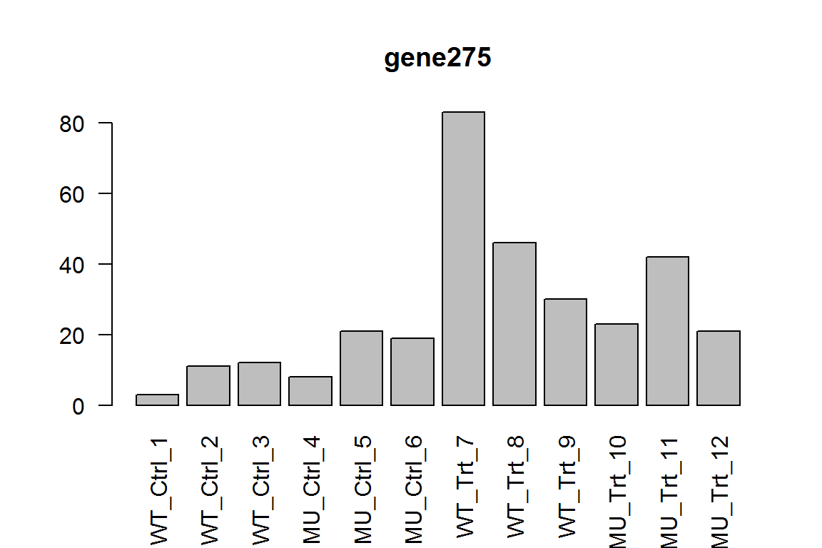
This is for WT, treated compared with untreated. Note that WT is not mentioned, because it is the reference level. In other words, this is the difference between samples No. 7-9, compared with samples No. 1-3.
Here we show the most significant gene.
barplot(assay(dds)[ix,],las=2, main=rownames(dds)[ ix ] )
##The effect of treatment in mutant This is, by definition, the main effect plus the interaction term (the extra condition effect in genotype Mutant compared to genotype WT).
res <- results(dds, list( c("condition_Trt_vs_Ctrl","genotypeMU.conditionTrt") ))
ix = which.min(res$padj) # most significant
res <- res[order(res$padj),] # sort
kable(res[1:5,-(3:4)])
| baseMean | log2FoldChange | pvalue | padj | |
|---|---|---|---|---|
| gene5102 | 18.69017 | 4.757057 | 1.60e-06 | 0.0156912 |
| gene7367 | 170.69259 | 1.481016 | 1.19e-05 | 0.0396827 |
| gene8351 | 27.77227 | 3.033622 | 9.80e-06 | 0.0396827 |
| gene8034 | 53.34342 | -1.841023 | 1.62e-05 | 0.0403724 |
| gene7272 | 92.82351 | -1.414967 | 6.70e-05 | 0.1125817 |
Note that it has to be list( c(“condition_Trt_vs_Ctrl”,“genotypeMU.conditionTrt”) ). If list( ) is ommitted, the results would be drastically different. Perhaps only the first coefficient is used.
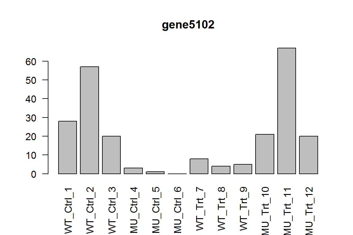
This measures the effect of treatment in mutant. In other words, samples No. 10-12 compared with samples No. 4-6.
Here we show the most significant gene, which is downregulated expressed in samples 10-12, than samples 4-6 , as expected.
barplot(assay(dds)[ix,],las=2, main=rownames(dds)[ ix ] )

##What is the difference between mutant and wild-type without treatment?
As Ctrl is the reference level, we can just retrieve the “genotype_MU_vs_WT”.
res = results(dds, contrast=c("genotype","MU","WT"))
ix = which.min(res$padj) # most significant
res <- res[order(res$padj),] # sort
kable(res[1:5,-(3:4)])
| baseMean | log2FoldChange | pvalue | padj | |
|---|---|---|---|---|
| gene5102 | 18.69017 | -4.714519 | 0.0000020 | 0.0195596 |
| gene2289 | 45.04711 | 1.763615 | 0.0000333 | 0.1218107 |
| gene3388 | 122.85582 | -1.529323 | 0.0000366 | 0.1218107 |
| gene915 | 39.03250 | 2.104003 | 0.0001133 | 0.2374861 |
| gene8351 | 27.77227 | -2.653182 | 0.0001190 | 0.2374861 |
In other words, this is the samples No.4-6 compared with No. 1-3. Here we show the most significant gene.
barplot(assay(dds)[ix,],las=2, main=rownames(dds)[ ix ] )
##With treatment, what is the difference between mutant and wild-type?
res = results(dds, list( c("genotype_MU_vs_WT","genotypeMU.conditionTrt") ))
ix = which.min(res$padj) # most significant
res <- res[order(res$padj),] # sort
kable(res[1:5,-(3:4)])
| baseMean | log2FoldChange | pvalue | padj | |
|---|---|---|---|---|
| gene4127 | 50.03677 | 1.925094 | 0.0000091 | 0.0910879 |
| gene3879 | 34.67704 | -2.133203 | 0.0000283 | 0.0940393 |
| gene4799 | 24.11059 | -2.459345 | 0.0000197 | 0.0940393 |
| gene5441 | 58.67469 | -1.744769 | 0.0001418 | 0.2357639 |
| gene5926 | 161.16737 | 1.524163 | 0.0001339 | 0.2357639 |
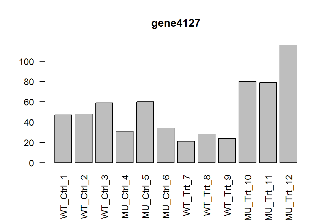
This gives us the difference between genotype MU and WT, under condition Trt. In other words, this is the sampless No. 10-12 compared with samples 7-9.
Here we show the most significant gene.
barplot(assay(dds)[ix,],las=2, main=rownames(dds)[ ix ] )
The different response in genotypes (interaction term)
Is the effect of treatment different across genotypes? This is the interaction term.
res = results(dds, name="genotypeMU.conditionTrt")
ix = which.min(res$padj) # most significant
res <- res[order(res$padj),] # sort
kable(res[1:5,-(3:4)])
| baseMean | log2FoldChange | pvalue | padj | |
|---|---|---|---|---|
| gene5102 | 18.69017 | 7.395771 | 0.0000000 | 0.0000341 |
| gene5441 | 58.67469 | -3.297673 | 0.0000004 | 0.0019104 |
| gene8034 | 53.34342 | -2.564030 | 0.0000205 | 0.0682558 |
| gene8858 | 14.68650 | 4.703936 | 0.0000297 | 0.0742076 |
| gene4799 | 24.11059 | -2.990101 | 0.0001234 | 0.2463661 |
Here we show the most significant gene.
barplot(assay(dds)[ix,],las=2, main=rownames(dds)[ ix ] )

In wild-type, this gene is upregulated by treatment, while for the mutant, it is downregulated.
Example 4: Two conditionss, three genotpes with interaction terms
dds <- makeExampleDESeqDataSet(n=10000,m=18)
dds$genotype <- factor(rep(rep(c("I","II","III"),each=3),2))
colnames(dds) <- paste(rownames(colData(dds)), as.character( dds$condition), as.character( dds$genotype),sep="_"  )
colnames(dds) = gsub("sample","S",colnames(dds))
design(dds) <- ~ genotype + condition + genotype:condition
dds <- DESeq(dds)
kable( colData(dds))
| condition | genotype | sizeFactor | |
|---|---|---|---|
| S1_A_I | A | I | 1.053964 |
| S2_A_I | A | I | 1.058935 |
| S3_A_I | A | I | 1.061629 |
| S4_A_II | A | II | 1.047347 |
| S5_A_II | A | II | 1.059813 |
| S6_A_II | A | II | 1.049639 |
| S7_A_III | A | III | 1.060271 |
| S8_A_III | A | III | 1.057331 |
| S9_A_III | A | III | 1.052053 |
| S10_B_I | B | I | 1.053989 |
| S11_B_I | B | I | 1.044408 |
| S12_B_I | B | I | 1.042376 |
| S13_B_II | B | II | 1.042354 |
| S14_B_II | B | II | 1.050094 |
| S15_B_II | B | II | 1.045868 |
| S16_B_III | B | III | 1.050772 |
| S17_B_III | B | III | 1.047934 |
| S18_B_III | B | III | 1.036983 |
resultsNames(dds)
## [1] "Intercept"              "genotype_II_vs_I"
## [3] "genotype_III_vs_I"      "condition_B_vs_A"
## [5] "genotypeII.conditionB"  "genotypeIII.conditionB"
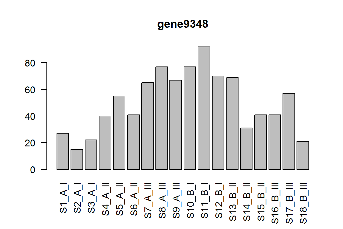
The condition effect for genotype I (the main effect)
res = results(dds, contrast=c("condition","B","A"))
ix = which.min(res$padj) # most significant
res <- res[order(res$padj),] # sort
kable(res[1:5,-(3:4)])
| baseMean | log2FoldChange | pvalue | padj | |
|---|---|---|---|---|
| gene9348 | 48.01943 | 1.915941 | 0.0000155 | 0.1546441 |
| gene928 | 60.03093 | -1.562622 | 0.0001151 | 0.5748158 |
| gene931 | 439.23135 | -1.101161 | 0.0004187 | 0.6066182 |
| gene4483 | 16.83153 | 2.957899 | 0.0005487 | 0.6066182 |
| gene4612 | 29.09139 | -1.742999 | 0.0006893 | 0.6066182 |
barplot(assay(dds)[ix,],las=2, main=rownames(dds)[ ix ] )
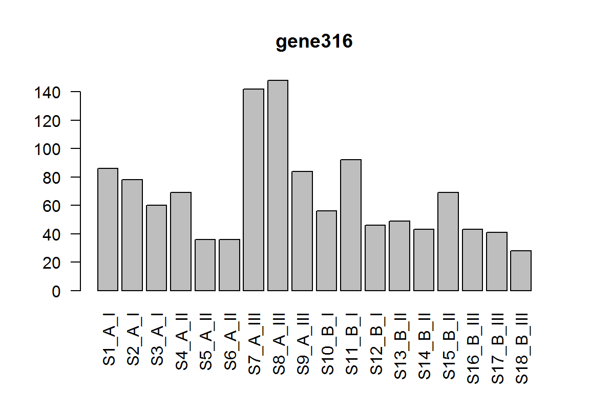
The condition effect for genotype III.
This is the main effect plus the interaction term (the extra condition effect in genotype III compared to genotype I).
res = results(dds, contrast=list( c("condition_B_vs_A","genotypeIII.conditionB") ))
ix = which.min(res$padj) # most significant
res <- res[order(res$padj),] # sort
kable(res[1:5,-(3:4)])
| baseMean | log2FoldChange | pvalue | padj | |
|---|---|---|---|---|
| gene316 | 63.666427 | -1.724235 | 0.0000294 | 0.2936262 |
| gene252 | 5.751827 | -6.012712 | 0.0001418 | 0.2977597 |
| gene2068 | 16.851863 | -2.725616 | 0.0001422 | 0.2977597 |
| gene6828 | 19.669827 | 2.840392 | 0.0000635 | 0.2977597 |
| gene7420 | 85.226424 | -1.510240 | 0.0001788 | 0.2977597 |
barplot(assay(dds)[ix,],las=2, main=rownames(dds)[ ix ] )
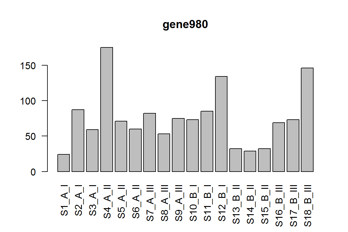
The condition effect for genotype II.
This is the main effect plus the interaction term (the extra condition effect in genotype II compared to genotype I).
res = results(dds, contrast=list( c("condition_B_vs_A","genotypeII.conditionB") ))
ix = which.min(res$padj) # most significant
res <- res[order(res$padj),] # sort
kable(res[1:5,-(3:4)])
| baseMean | log2FoldChange | pvalue | padj | |
|---|---|---|---|---|
| gene980 | 71.929692 | -1.711667 | 0.0005822 | 0.648323 |
| gene1177 | 109.057633 | -1.281177 | 0.0002111 | 0.648323 |
| gene5118 | 3.487054 | -5.757413 | 0.0005110 | 0.648323 |
| gene5570 | 23.786589 | 2.329791 | 0.0004286 | 0.648323 |
| gene6519 | 94.137270 | 1.422193 | 0.0001399 | 0.648323 |
barplot(assay(dds)[ix,],las=2, main=rownames(dds)[ ix ] )

This is equivalent to using numeric vector referencing to each of the results.
[1] “Intercept” “genotype_II_vs_I” “genotype_III_vs_I”
[4] “condition_B_vs_A” “genotypeII.conditionB” “genotypeIII.conditionB”
res = results(dds, contrast= c(0,0,0,1,1,0))
ix = which.min(res$padj) # most significant
res <- res[order(res$padj),] # sort
kable(res[1:5,-(3:4)])
| baseMean | log2FoldChange | pvalue | padj | |
|---|---|---|---|---|
| gene980 | 71.929692 | -1.711667 | 0.0005822 | 0.648323 |
| gene1177 | 109.057633 | -1.281177 | 0.0002111 | 0.648323 |
| gene5118 | 3.487054 | -5.757413 | 0.0005110 | 0.648323 |
| gene5570 | 23.786589 | 2.329791 | 0.0004286 | 0.648323 |
| gene6519 | 94.137270 | 1.422193 | 0.0001399 | 0.648323 |
barplot(assay(dds)[ix,],las=2, main=rownames(dds)[ ix ] )
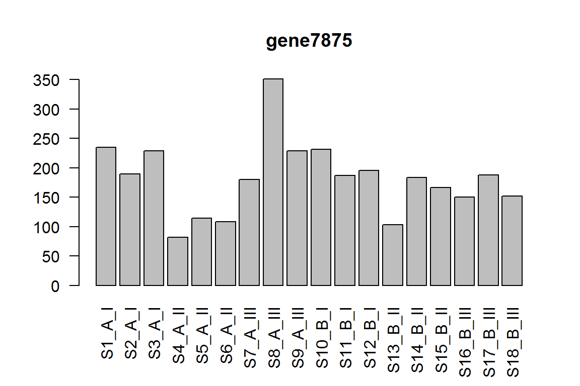
The effect of III vs. II, under condition A.
This is the effect of “genotype_III_vs_I” minus “genotype_II_vs_I” ?
res = results(dds, contrast= c(0,-1,1,0,0,0))
ix = which.min(res$padj) # most significant
res <- res[order(res$padj),] # sort
kable(res[1:5,-(3:4)])
| baseMean | log2FoldChange | pvalue | padj | |
|---|---|---|---|---|
| gene7875 | 172.84101 | 1.316870 | 0.0000354 | 0.3541800 |
| gene316 | 63.66643 | 1.399247 | 0.0006044 | 0.5256726 |
| gene557 | 17.92683 | -1.980097 | 0.0008418 | 0.5256726 |
| gene1243 | 51.92628 | -1.844387 | 0.0004523 | 0.5256726 |
| gene1702 | 55.34857 | -1.631481 | 0.0006698 | 0.5256726 |
barplot(assay(dds)[ix,],las=2, main=rownames(dds)[ ix ] )
The interaction term for condition effect in genotype III vs genotype I.
This tests if the condition effect is different in III compared to I
res = results(dds, name="genotypeIII.conditionB")
ix = which.min(res$padj) # most significant
res <- res[order(res$padj),] # sort
kable(res[1:5,-(3:4)])
| baseMean | log2FoldChange | pvalue | padj | |
|---|---|---|---|---|
| gene9348 | 48.019429 | -2.714891 | 0.0000104 | 0.1042074 |
| gene6251 | 14.477069 | -4.780646 | 0.0000479 | 0.2395245 |
| gene839 | 161.393935 | -1.662756 | 0.0000886 | 0.2950638 |
| gene9383 | 9.149222 | -6.436304 | 0.0001560 | 0.3896367 |
| gene931 | 439.231351 | 1.562204 | 0.0003858 | 0.4506833 |
barplot(assay(dds)[ix,],las=2, main=rownames(dds)[ ix ] )

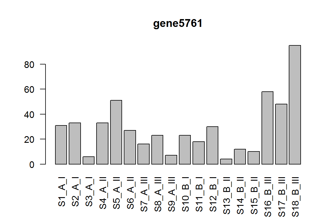
The interaction term for condition effect in genotype III vs genotype II.
This tests if the condition effect is different in III compared to II
res = results(dds, contrast=list("genotypeIII.conditionB", "genotypeII.conditionB"))
ix = which.min(res$padj) # most significant
res <- res[order(res$padj),] # sort
kable(res[1:5,-(3:4)])
| baseMean | log2FoldChange | pvalue | padj | |
|---|---|---|---|---|
| gene5761 | 27.797507 | 4.231182 | 0.0000012 | 0.0116510 |
| gene6598 | 100.143591 | 2.317486 | 0.0000214 | 0.1068006 |
| gene3491 | 325.224707 | 1.942243 | 0.0001168 | 0.2853814 |
| gene4635 | 8.411707 | 5.206116 | 0.0000963 | 0.2853814 |
| gene5118 | 3.487054 | 8.088922 | 0.0002454 | 0.2853814 |
barplot(assay(dds)[ix,],las=2, main=rownames(dds)[ ix ] )
Example 5: Three conditions, three genotypes with interaction terms
For a more complex example, we now have a 3x3 factorial design. It is convenent to use a diagram to represent study design and the coefficients generated by DESeq2. Each connections in the diagram below represents a coefficient for a contrast and we can use the combination of these to define desired contrasts by travelling through the graph/network.

dds <- makeExampleDESeqDataSet(n=10000,m=18)
dds$genotype <- factor(rep(rep(c("I","II","III"),each=3),2))
dds$condition <-factor(rep(c("A","B","C"), 6)  )
colnames(dds) <- paste(as.character( dds$genotype), as.character( dds$condition),rownames(colData(dds)), sep="_"  )
colnames(dds) = gsub("sample","",colnames(dds))
design(dds) <- ~ genotype + condition + genotype:condition
dds <- DESeq(dds)
kable( colData(dds))
| condition | genotype | sizeFactor | |
|---|---|---|---|
| I_A_1 | A | I | 1.055853 |
| I_B_2 | B | I | 1.037228 |
| I_C_3 | C | I | 1.048146 |
| II_A_4 | A | II | 1.048901 |
| II_B_5 | B | II | 1.062858 |
| II_C_6 | C | II | 1.036711 |
| III_A_7 | A | III | 1.052625 |
| III_B_8 | B | III | 1.033361 |
| III_C_9 | C | III | 1.040028 |
| I_A_10 | A | I | 1.054525 |
| I_B_11 | B | I | 1.045331 |
| I_C_12 | C | I | 1.036150 |
| II_A_13 | A | II | 1.052502 |
| II_B_14 | B | II | 1.047103 |
| II_C_15 | C | II | 1.063802 |
| III_A_16 | A | III | 1.053762 |
| III_B_17 | B | III | 1.041255 |
| III_C_18 | C | III | 1.048660 |
resultsNames(dds)
## [1] "Intercept"              "genotype_II_vs_I"
## [3] "genotype_III_vs_I"      "condition_B_vs_A"
## [5] "condition_C_vs_A"       "genotypeII.conditionB"
## [7] "genotypeIII.conditionB" "genotypeII.conditionC"
## [9] "genotypeIII.conditionC"
To derive desired contrasts, we can travel on the network of factor levels, using the given 9 coefficients as bridges.For example, we are interested in the difference between genotpes III vs. II, under condition C. This is not readily available. But we can travel from C to III, then III to I, I to II, and then II to C. Namely the path is C–III–I–II–C. In terms of coefficients: (III-I) - (II-I) + III.C - II.C= “genotype_III_vs_I” - “genotype_II_vs_I” + “genotypeIII.conditionC” - “genotypeII.conditionC” For such a complex contrast, we can use the numerical combination using a vector: c(0,-1,1,0,0,0,0,-1,1 ) These numbers are applied to the coefficients in the resultsNames. To double check we order them:
cbind(resultsNames(dds),c(0,-1,1,0,0,0,0,-1,1 ) )
##       [,1]                     [,2]
##  [1,] "Intercept"              "0"
##  [2,] "genotype_II_vs_I"       "-1"
##  [3,] "genotype_III_vs_I"      "1"
##  [4,] "condition_B_vs_A"       "0"
##  [5,] "condition_C_vs_A"       "0"
##  [6,] "genotypeII.conditionB"  "0"
##  [7,] "genotypeIII.conditionB" "0"
##  [8,] "genotypeII.conditionC"  "-1"
##  [9,] "genotypeIII.conditionC" "1"
Now we can extract the contrast.
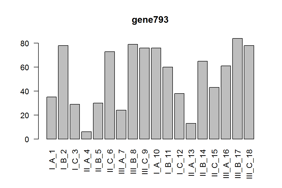
The effect of III vs. II, under condition C.
res = results(dds, contrast= c(0,-1,1,0,0,0,0,0,1 ))
ix = which.min(res$padj) # most significant
res <- res[order(res$padj),] # sort
kable(res[1:5,-(3:4)])
| baseMean | log2FoldChange | pvalue | padj | |
|---|---|---|---|---|
| gene793 | 50.368566 | 3.737810 | 3.36e-05 | 0.1460573 |
| gene1161 | 827.243573 | 1.844200 | 4.39e-05 | 0.1460573 |
| gene3314 | 23.430794 | 4.580687 | 1.57e-05 | 0.1460573 |
| gene4445 | 51.054925 | -3.096770 | 6.96e-05 | 0.1736784 |
| gene1555 | 5.073803 | 10.771498 | 9.70e-05 | 0.1937244 |
barplot(assay(dds)[ix,],las=2, main=rownames(dds)[ ix ] )
How about many factors, each with many levels? It’s going to become increasingly complex. Drawing a network graph like the one above can help you find the right combination.
Please let me know if you have any comment.